The most popular learning algorithm for forward connection networks is back-propagation algorithm. This a.lgorithm defines the sum of squared errors measured on the output layer as the error function and updates weights to minimize this error by the steepest descent method. This adaptation of the learning rate during learning has been shown to significantly improve the convergence rate of the back-propagation algorithm.
List of Tables
INTRODUCTION
General Introduction
The underlying reason is that, unlike conventional computers, the brain contains a large number of neurons—the information-processing elements of the biological nervous system—that work in parallel. But artificial neural network models are not meant to duplicate, but to abstract a few properties from what is known about brain function based on current understanding of the biological nervous system.
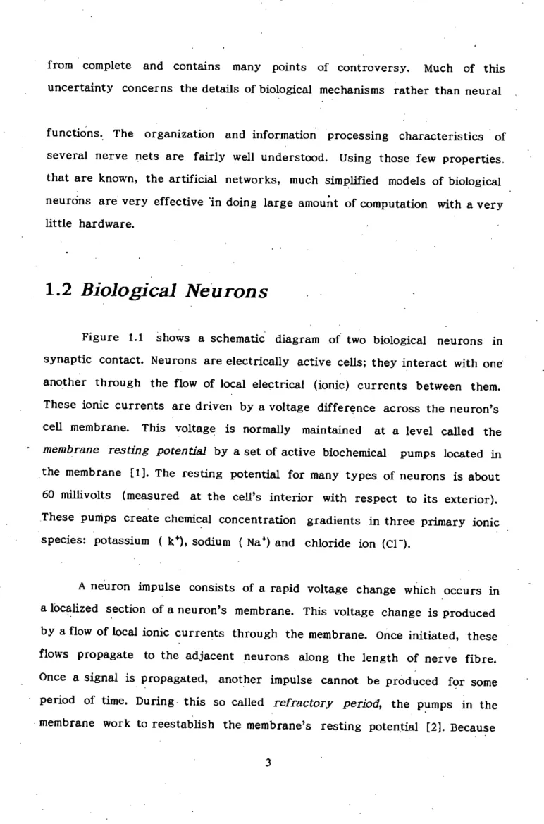
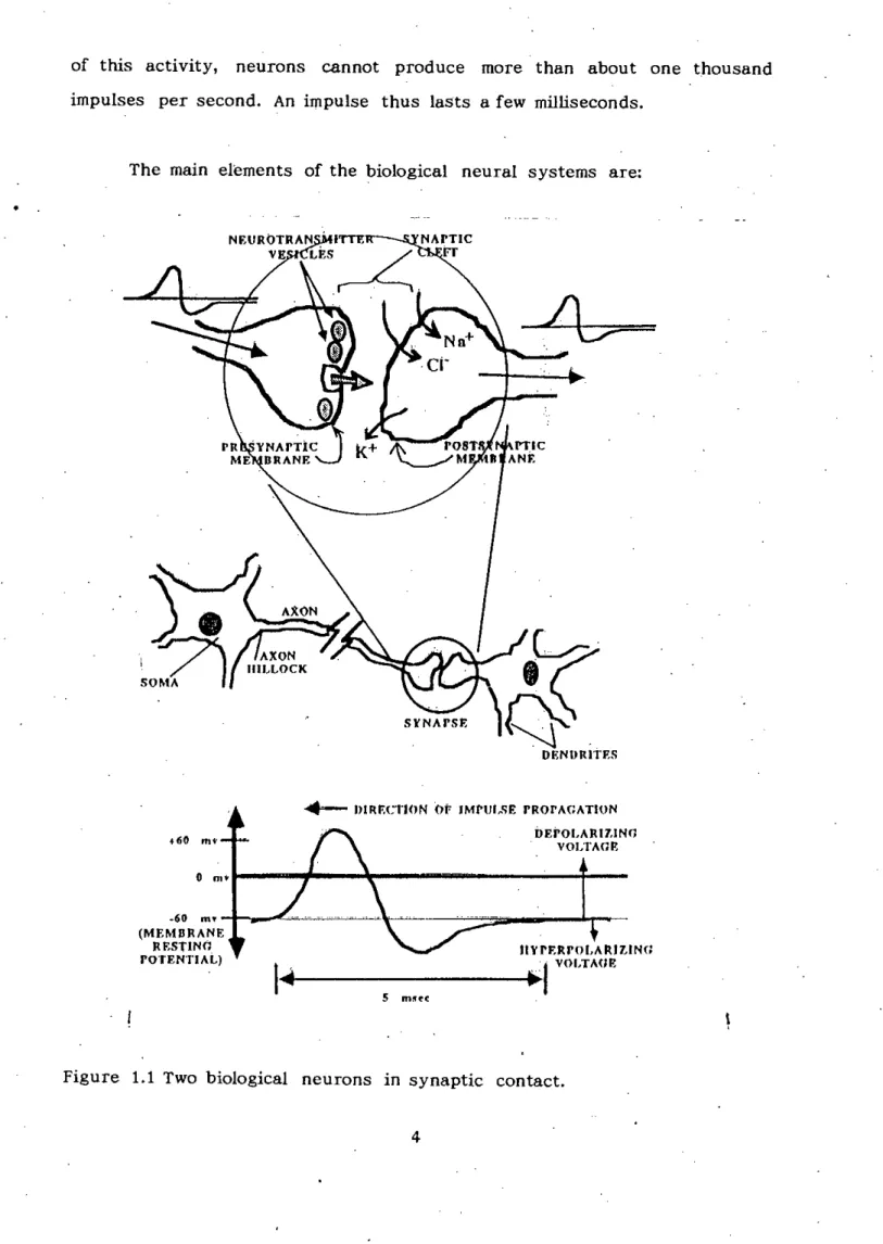
Biological Neurons
The input fiber leading to the soma, called the dendrite, receives input from other neurons by means of specialized contacts. Neurons can combine impulses reaching them from other neurons into two integrative effects called temporal summation and spatial summation [3].
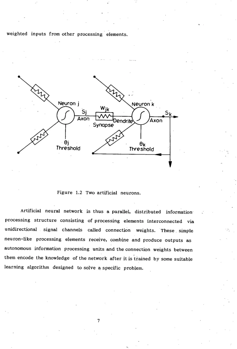
Artificial Neural Networks
Some of these inputs can be so powerful that impulses coming from individual inputs can be enough to cause the receiving cell to fire. Each neuron receives, combines and produces impulses as an autonomous information processing unit, operating in parallel with other neurons.
Axon
Potential Applications of Neural Networks
DESKNET's neural network-based diagnostic system can diagnose 10 different skin diseases based on a set of 18 symptoms and test results. British Telecom, American Telegraph and Telecom (AT&T), and Nippon Telegraph and Telecom (NTT) are designing applications that use neural network-based speech processing, recognition, and synthesis.
Scope of the Present Work
Thesis Organization
CHAPTER. 2
BACK-PROPAGATION LEARNING. ALGORITHM
- Intioduction
- Formulation of Back-propagation
- Update of Output-layer weight
- Update of Hidden-layer Weight
- Limitations Standard Back-propagation algorithm
- Reasons for slow convergence
- Summary
Backpropagation is one of the most commonly used algorithms for training multi-layer forward networks. When the network receives input, the update of the activation values propagates forward from the input layer of the processing units, through each inner layer, often called the hidden layer, to the output layer of the processing units. The error at each output unit is Ypk-O pk', where Ypk is the desired output value of the kth output unit.
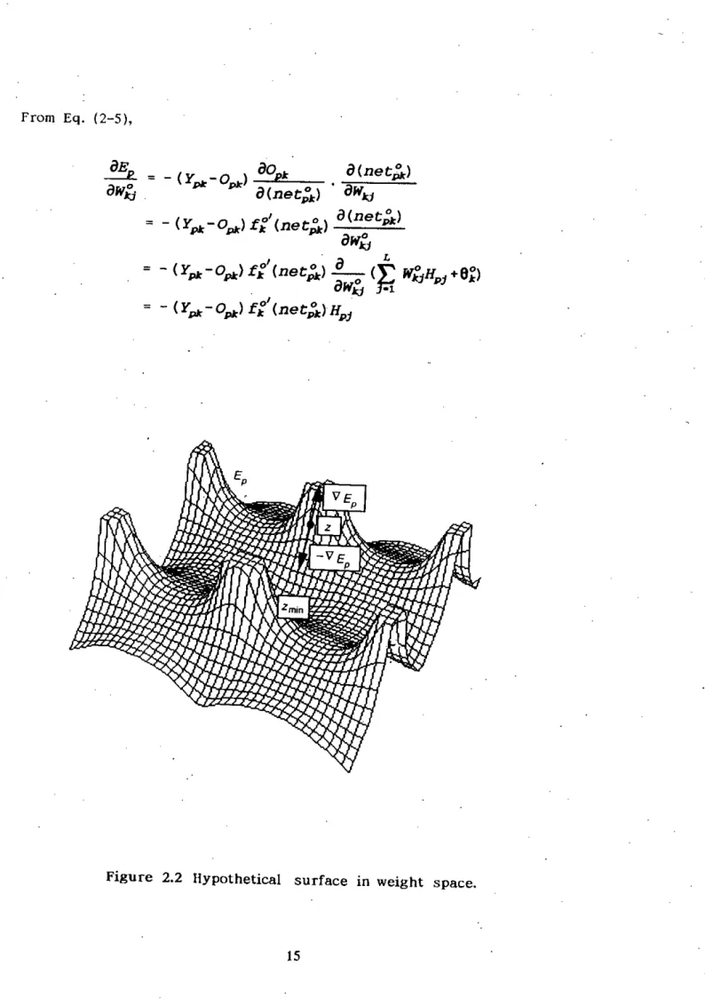
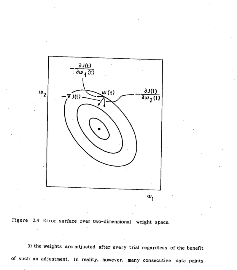
The error minimized by the gradient descent rule is the sum of the squares of the errors for all outputs. To determine the direction to change. weights, the negative of the gradient of Ep' OEp' with respect to the weights Wkjare to be calculated. Then the values of the weights can be adjusted so that the overall error is reduced.
To extend the above weight update procedure in the hidden layer, it is necessary to determine a measure of the error of the output of the hidden layer units.

PREVIOU S WORKS ON ACCELERATED CONVERGENCE
Introd~ction
The single biggest obstacle to the widespread use of the back-propagation learning algorithm in real-world applications is its slow rate of convergence, and it scales up poorly as tasks become larger and more complex. Even for relatively simple problems, standard back-propagation often requires a lengthy training process, where the complete set of training examples is processed hundreds or thousands of times. Some important real-world problems can be solved using networks of this size, but most of the tasks for which connection technology may be appropriate are far too large and complex to be handled by current training algorithms.
Much of the effort in neural network research is devoted to the development of faster convergent algorithms.
Survey of Previous _Works
Third, when the derivative of error with respect to a weight possesses the same sign for several consecutive iterations, its learning rate must be Increased learning rate for this weight can reduce the number of time steps required to travel this distance. Fourth, when the sign of the derivative for a weight varies for several consecutive time steps, its learning rate must be reduced.
This is often the case where the error surface along the weight dimension has a high curvature and therefore the slope of this area of the error surface can change sign rapidly. Based on the above consideration, Jacobs proposed individual learning rate for each weight and updating this learning rate on an estimate of the curvature of error surface at the current point along that weight. The reason is that, to update a specific weight, Backpropagation takes gradient on an error surface assuming all other weights are stationary.
A limitation of this new cost function is that it cannot be used in applications where linear devices are needed at the output layer.
Summary
CHAPTER-4
PROPOSED ACCELERATION TECHNIQUE
Proposed Cost Function
Based on the analysis of the causes of slow convergence in the backpropagation algorithm, presented in the previous chapter, a new cost function is proposed in order to achieve accelerated convergence. With this cost function, the effective learning rate parameter changes as a function of the error rate.
Weight Updating Using Proposed Cost Function
- Further "Modification
A close observation of equation (4-3) shows that the term l3eBEP must be calculated each time a pattern is presented. The computational overhead using the proposed cost function can be reduced if the term J3eBEpis is replaced or approximated by l3eBE where E is defined in equation (2-7). Then this term only needs to be calculated once for each training cycle and can be used for the presentation of each pattern.
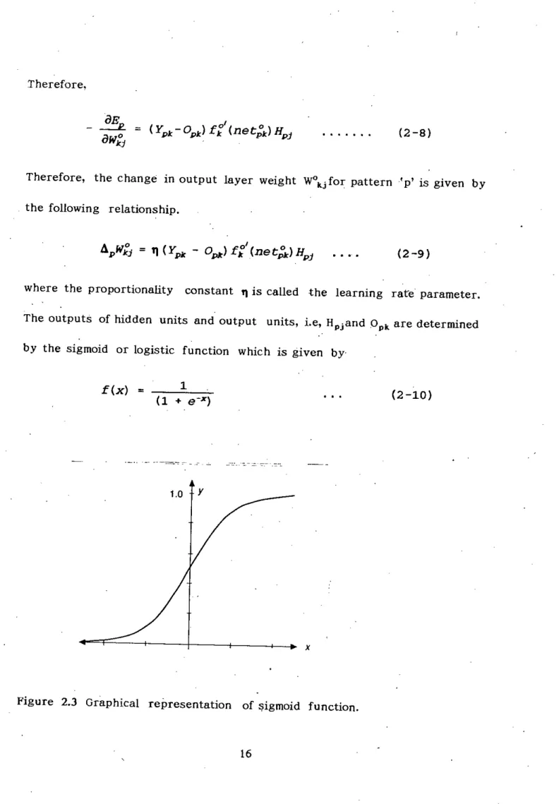
II-efixes the learning speed parameter in the standard Back-propagation II multiplied by a factor that is an exponential function of the error measure in the output layer. This will keep the learning rate high at the beginning and low in the final phase of learning and adjust the error rate as needed. 10] using the Log-lihood cost function eliminates the 0pk(l-Opk) term in the output layer weight update equation.
It would be interesting to see how the elimination of the above term in the weight update equation [equation (4-4)] plays out.
Summary
CHAPTER-5
SIMULATION RESULTS
Introduction
To investigate the convergence behavior and speed of the proposed modification -in the previous chapter, simulations are performed with different types of problems. Since there are no analytical techniques available to study the convergence of Back-propagation algorithm, simulation. The first is the XOR problem, which is treated as a benchmark problem in the neural network literature and has been used to test the modifications proposed in [5]-[12].
In this case, both -input and target are analog values instead of binary values used in the previous ones. In the following sections, the results of the simulation with the proposed modification and performance comparison with standard Back-propagation are presented.
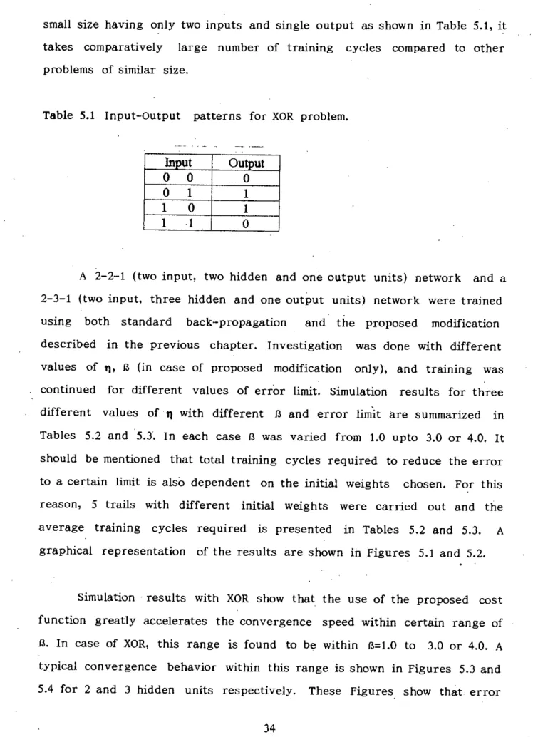
XOR Problem
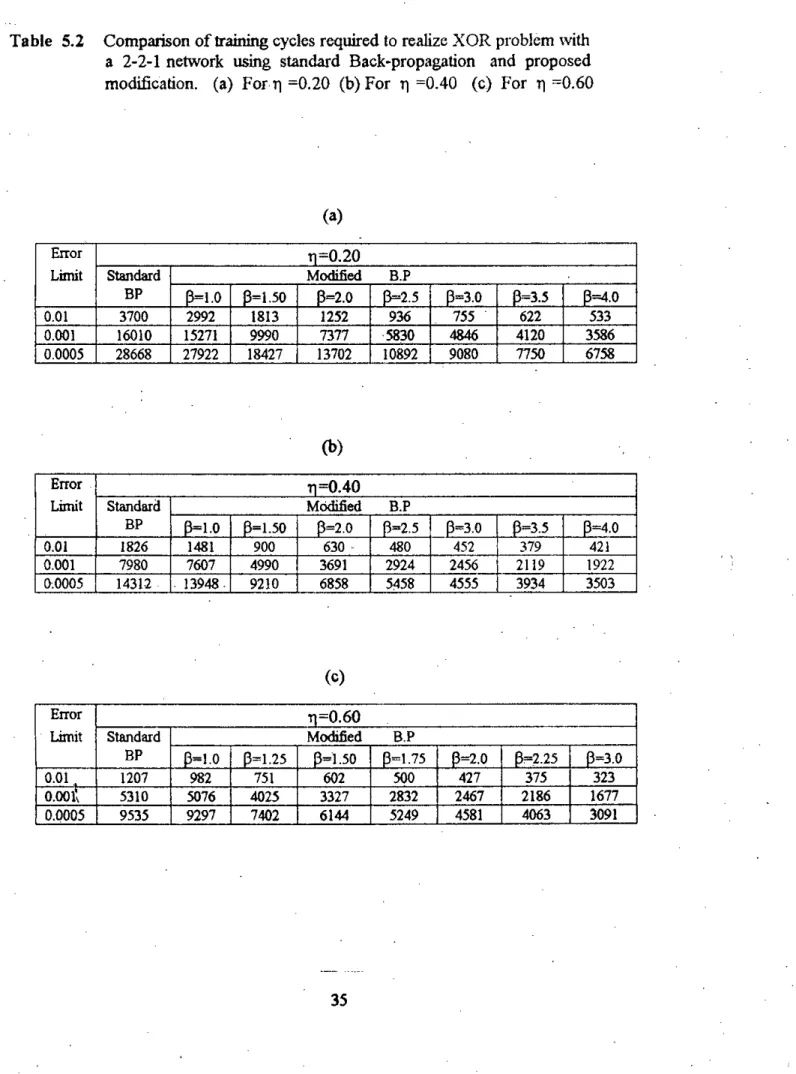
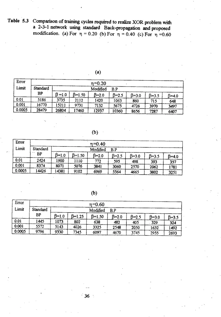
A 2-2-1 (two inputs, two hidden and one output units) network and a 2-3-1 (two inputs, three hidden and one output units) network were trained using both standard back-propagation and the proposed modification described in the previous chapter. The study was performed with different values of t), 13 (only in case of proposed change) and training was continued for different values of error bound. Simulation results for three different values often) with different 13 and error bounds are summarized in Tables 5.2 and 5.3.
It should be mentioned that the total number of training cycles required to reduce the error to a certain limit also depends on the initial weights chosen. For this reason, 5 courses with different initial weights were performed and the average training cycles required are shown in Tables 5.2 and 5.3. A typical convergence behavior within this range is shown in Figures 5.3 and 5.4 for 2 and 3 hidden units, respectively.
1000 Cycles
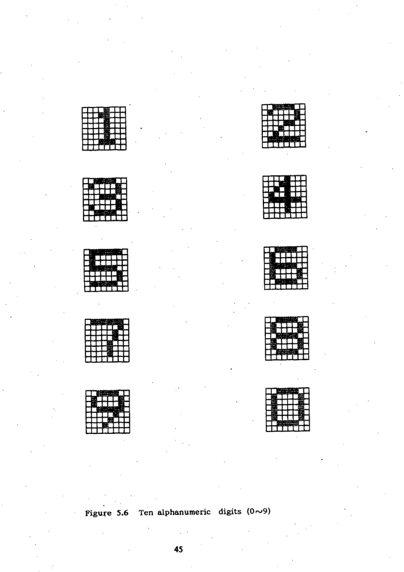
Character Recognition Problem
A network with 64 input units, 10 output units and 5 hidden units (64-5-10) and a (64-6-10) network were trained using standard backpropagation and proposed modifications. The networks were trained with different values of I and 13. For each set of I and 13, 5 routes were created. Simulation results showing the average training cycles required to reduce errors to a certain limit are summarized in Tables 5.5 and 5.6.
The results show that the convergence is significantly faster when the modified back-propagation is used with a value of 13 within a certain limit. On the other hand, as Figure 5.10 shows, an appropriate combination of I and 13 provides a smooth learning process, resulting in faster convergence. Ultimately, the learning rate and error reduction follow a smooth variation in the final learning phase.
As done in XOR, WiiS also investigated the character recognition problem using the Log-likelihood cost function and the modification proposed in Eq.(4-9) simulation results for different values of , .
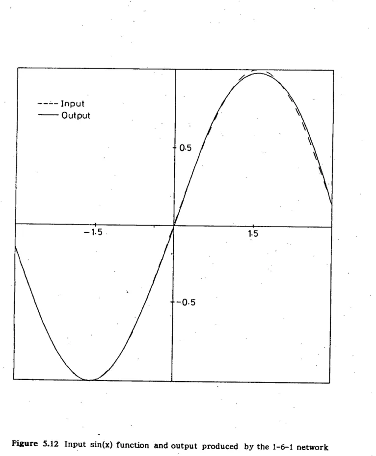
Function Approximation
Here too, for 13 approximately within the range of 1.0N 1.5, the modification significantly accelerates the convergence speed. Modification takes only half the number of training cycles required by standard Backpropagation. Since suitable value of 'I for good convergence is problem specific, the value of '1=0.20 appears to be large for .standard Backpropagation and therefore causes oscillation.
Summary
CONCLUSION
Conclusion
Standard Backpropagation uses the sum of squared error measured at output layer as the cost function and updates weights to minimize this error in the steepest descent method. In the present work, a new cost function is defined as an exponential function of the sum of squared error measured at the output layer. Simulation results with two problems having a binary input-output relationship and one problem having an analog input-output relationship show significant improvement in convergence speed within certain suitable range of 13. As 'I in standard Backpropagation, choice of suitable range of 13 yielding accelerated convergence is also problem specific.
In the simulation, it was found that in cases where a certain value of 1) which causes a large fluctuation in learning with standard backpropagation, allows smooth learning in the proposed modification with a suitable value of 13. This is because the modification adjusts the effective learning rate during training . Thus, a suitable pick 13 in this modification is just as crucial as pick 1) in the standard back spread. By observing the simulation results, a range of 13 is recommended in this study.
In situations where one has to train many candidate networks, training networks with Baround, once a suitable value of B is found, can thus save considerable computational time.
Future Work
APPENDIX