PREDICTING ABSENTEEISM OF EMPLOYEES AT WORKPLACE USING TREE-BASED
ALGORITHMS
By
ZAMAN WAHID (151-35-953)
A thesis submitted in partial fulfillment of the requirement for the degree of Bachelor of Science in Software Engineering
Department of Software Engineering DAFFODIL INTERNATIONAL UNIVERSITY
Fall – 2018
APPROVAL
This thesis titled on “Predicting Absenteeism of Employees at Workplace Using Tree-Based Algorithms”, submitted by Zaman Wahid, 151-35-953 to the Department of Software Engineering, Daffodil International University has been accepted as satisfactory for the partial fulfillment of the requirements for the degree of Bachelor of Science in Software Engineering and approval as to its style and contents.
BOARD OF EXAMINERS
--- Dr. Touhid Bhuiyan
Professor and Head
Department of Software Engineering
Faculty of Science and Information Technology Daffodil International University
Chairman
--- K. M. Imtiaz-Ud-Din
Assistant Professor
Department of Software Engineering
Faculty of Science and Information Technology Daffodil International University
Internal Examiner 1
--- Asif Khan Shakir
Lecturer
Department of Software Engineering
Faculty of Science and Information Technology Daffodil International University
Internal Examiner 2
--- Dr. Md. Nasim Akhtar
Professor Department of Computer Science and Engineering
Faculty of Electrical and Electronic Engineering
Dhaka University of Engineering & Technology, Gazipur
External Examiner
DECLARATION
It hereby declere that this thesis has been done by me, Zaman Wahid under the supervision of Dr. Touhid Bhuiyan, Professor and Head, Department of Software Engineering, Daffodil International University. It also declere that neither this thesis nor any part of this has been submitted elesewhere for award of any degree.
_______________________
Student Name: Zaman Wahid Student ID: 151-35-953
Batch: 16th
Department of Software Engineering
Faculty of Science & Information Technology Daffodil International University
Certified by:
_________________________
Dr. Touhid Bhuiyan Professor and Head
Department of Software Engineering
Faculty of Science & Information Technology Daffodil International University
ACKNOWLEDGEMENT
Firstly I express my sincere gratitude to Almighty Allah for blessing me with good health and peaceful mind during the whole process of this research. Thus to complete the final year thesis successfully in order to achieve the degree of Bachelor of Science in Software Engineering under the Faculty of Science and Technology, Daffodil International University.
I am really happy and grateful, and convey my profound respect and gratitude to Dr.
Touhid Bhuiyan, Professor and Head, Department of Software Engineering, Daffodil International University, for investing his keen interest as my supervisor and deep knowledge in machine learning and employee management at workplace to carry out this thesis to success. His scholarly guidance, endless patience and encouragement, constructive criticism, and reviewing from document to experiment on stage made it successful to finish this thesis in time while leaving behind thousand opportunities to further this thesis.
Finally I am thankful to all other faculty members, staffs, and resources of Department of Software Engineering for making this journey smoother.
TABLE OF CONTENT
APPROVAL ...i
DECLARATION ... ii
ACKNOWLEDGEMENT ...iv
TABLE OF CONTENT ... v
LIST OF TABLE ... vii
LIST OF FIGURE ... viii
ABSTRACT ...ix
CHAPTER 1: INTRODUCTION ... 1
1.1 Background ... 1
1.2 Motivation of the Research ... 2
1.3 Problem Statement ... 2
1.4 Research Questions ... 2
1.5 Research Objectives ... 3
1.6 Research Scope ... 3
1.7 Thesis Organization ... 3
CHAPTER 2: LITERATURE REVIEW ... 5
CHAPTER 3: METHODOLOGY ... 9
3.1 Tools and Techniques ... 10
3.2 Description of Dataset ... 11
3.3 Data Preprocessing ... 14
3.4 Partitioning ... 16
3.5 Classification ... 17
3.5.1 Decision Tree ... 18
3.5.2 Gradient Boosted Tree ... 21
3.5.3 Random Forest ... 23
3.6 Summary of this Chapter ... 25
CHAPTER 4: RESULTS AND DISCUSSION ... 26
4.1 Evaluation ... 26
4.2 Analysis ... 28
CHAPTER 5: CONCLUSIONS AND RECOMMENDATIONS ... 34
5.1 Findings and Contributions ... 34
5.2 Recommendations for Future Works ... 35
REFERENCES ... 36
Appendix A Parameters of Absenteeism at Work Dataset ... 39 LIST OF ABBREVIATION ... 43
LIST OF TABLE
Table 3.1: Reason for Absence with ICD ... 12
Table 3.2: Reason for Absence without ICD ... 13
Table 3.3: Code of Day of Week ... 13
Table 3.4: Code of Education ... 14
Table 3.5: Classification Rules of Absenteeism Time Class ... 15
Table 4.1: Data Analysis for Several Classifiers ... 30
LIST OF FIGURE
Figure 3.1: Research Methodology ... 9
Figure 3.2: Class Distribution after Applying Classification Rules ... 16
Figure 3.3: Decision Tree Model after Fitting the Dataset ... 20
Figure 3.4: Gradient Boosted Tree Model(15) after Fitting the Dataset ... 22
Figure 3.5: Gradient Boosted Tree Model(73) after Fitting the Dataset ... 22
Figure 3.6: Random Forest Model(1) after Fitting the Dataset ... 24
Figure 3.7: Random Forest Model(9) after Fitting the Dataset ... 25
Figure 4.1: Confusion Matrix of Decision Tree Model ... 28
Figure 4.2: Confusion Matrix of Gradient Boosted Tree Model ... 29
Figure 4.3: Confusion Matrix of Random Forest Model ... 29
Figure 4.4: Accuracy Score of Several Classifiers ... 32
Figure 4.5: Learning Model after Fitting the Dataset into Decision Tree ... 33
ABSTRACT
Absenteeism at workplace plays a crucial factor in demonstrating the productive and profitable capacity of a company. Thus the knowledge of absenteeism of employees’
becomes the principle for an organization in its multiple dimensions. Because the proper determination of employees’ profile allows the identification of excesses of occurrences of certain morbidities. The early absenteeism research primarily focused on predicting the characteristics and the categories of diseases of employees that make them perform higher absenteeism at workplace. However, predicting the absenteeism time of employees using tree-based machine learning classifiers and thus finding out the facts that should be taken into account to abate higher absenteeism at workplace are yet to be explored. In this thesis, we have applied three prominent machine learning algorithms namely Decision Tree, Gradient Boosted Tree, and Random Forest to predict absenteeism time of employees and to find out the insights that cause employees to perform higher absenteeism at work. Meanwhile comparing the different machine learning algorithms to find out the best classifier which produces the highest prediction accuracy. We have used an existing dataset of a courier company in Brazil in order to predict the absenteeism time of employees. The dataset contains 21 categories of the reason for absence which are attested by the International Classification of Disease (ICD) and 7 other categories without the ICD that have proved to be effective in detecting the absenteeism at work. We classified the absenteeism time into four categories such as NOT ABSENT, HOURS, DAYS, and WEEKS. Based on the seven evaluation metrics such as True Positive, True Negative, False Positive, False Negative, Sensitivity, Specificity, and Accuracy we have evaluated the model performance in predicting absenteeism at work. Our comparative analysis found that Gradient Boosted Tree produces the best result with an accuracy rate of 84.46% whereas Decision Tree performed the lowest with the accuracy rate of 80.41%. The Random Forest classifier performs in between with an accuracy rate of 82.43%. Using the tree model we discovered that the reason for absence class as diseases that are attested by International Code of Diseases (ICD), and the transportation expense from home to work are the topmost facts of performing higher absenteeism at workplace.
Keywords: Machine Learning, Absenteeism, Classification;
CHAPTER 1 INTRODUCTION
1.1 Background
The evolution of society underscored the importance of relationships between men, different cultures, and markets. Therefore, human labor has become more complex as the traditional sense of human labor is becoming supplanted to a means of satisfying needs. Absenteeism represents the loss of a productive and profitable capacity of a company. Absenteeism, in general, is defined as not work attendance as scheduled.
There is historically long research, since this phenomenon, in part, it generates a high cost for companies beyond their status of unfavorable indicators (Pal & Mather, 2003, p.554-565). It is also known as an expression used to denote the lack of interest to workplace, even not being motivated by prolonged illness or legal leave. The absence of employees in a working environment is considered as absenteeism which can be set temporary or permanent incapacity absence (Gayathri, 2018). In an organization, workability may decrease due to the characteristics of individuals such as lack of leisure time, vigorous physical activity, older age, lifestyle, high physical or psychological work demands, and physical condition, a systematic review of 20 empirical studies of determinants of workability revealed (Schouteten, 2017, p.52-57). Due to the shortage of employees, a service might be ceased which reduce the company’s credibility. A renowned research by the Gallup-Healthways Well-Being Index revealed that absenteeism at work and lost productivity cost over $40 billion a year in the US (The Causes & Cost of Absenteeism, 2013). It costs employers with both financially and mentally. The direct and indirect costs include absent employees’ wages, employee replacement costs, poor quality services and of course reduced productivity.
1.2 Motivation of the Research
I had chances of working at numerous organizations in both national and international level where I have been through diverse experiences in terms of productivity, working environment, and location. All those experiences filled me with a quest of understanding of the underlying facts of absenteeism at workplace. Additionally, understanding the causes and patterns of absenteeism of employees becomes fundamental for an organization in multiple dimensions as the proper determination of employees’ profile allows the identification of excesses of occurrences of certain morbidities. And if it could be achieved properly it would facilitate in improving companies productivity and credibility.
1.3 Problem Statement
The early studies limit the research within focusing on finding out the reason for absence, specifically the diseases that cause higher absenteeism, by developing a neuro- fuzzy network using Artificial Neural Network (ANN) algorithm only. However, there still remains plenty of unexplored options, especially applying tree-based algorithms to not only just predict absenteeism but also the overall factors that should be considered carefully. Meanwhile comparing the performance of different algorithms as well as finding out the better algorithms that produce higher prediction results.
1.3 Research Questions
1. How well tree-based algorithms perform in the prediction of absenteeism at workplace, and which one performs better?
2. What are the factors should be considered those cause employees to perform higher absenteeism?
1.5 Research Objectives
To apply three tree-based machine learning algorithms namely Decision Tree, Gradient Boosted Tree, and Random Forest that still remained unexplored mostly in these absenteeism research.
To find out the best classifier that produces higher accuracy in the prediction of absenteeism of employees at workplace.
To discover the factors that occur performing higher absenteeism at workplace
1.6 Research Scope
The scope of this research is limited to the employees of organizations in Brazil. The absenteeism data that have used in this research are based on a courier company in Brazil. Since only a few pieces of research which are solely focused on predicting absenteeism of employees have taken place for the last several years, there remains a plenty of opportunities to experiment with different machine learning algorithms on different country’s organizational data in line with improving the prediction results.
1.7 Thesis Organization
This thesis paper is organized into 8 sections for better explanation and understanding.
The following sections titled Literature Review, Description of Dataset, Methodology, Evaluation, Result and Analysis, Conclusions and Recommendations, and its’
subsections discuss this research from top to bottom in details. In the literature review section, the related works of absenteeism prediction have been described and summary of the research gap that we can leverage.
We described the attributes of the dataset in the next section. The detail description of the tools and techniques we have used to conduct this experiment is discussed in the methodology section. In the evaluation section, the metrics we have used to evaluate
the best classifier is described. Based on the evaluation metrics we scrutinized results in order to make decisions in the result and analysis section. The research is concluded with highlighting future works in the last section.
CHAPTER 2
LITERATURE REVIEW
To find out and understand the other researches related to absenteeism prediction at work we have studied several research papers. In the following sections, each of them is described.
Martiniano et al. (2012, p.1-4) developed a neuro-fuzzy network using a multilayer perceptron with the error back-propagation algorithm to predict absenteeism at work.
They collected the records of absenteeism from work of employees of a courier company during the period of July 2007 to July 2010. After tabulating and filtering the data, they classified the data of absences certified with the International Classification of Diseases (ICD) into 21 categories with the intention of obtaining the impact of these absences. They identified the six categories in the database together are the reason of 78.65% absences attested with ICD. They observed that category XIX, injuries, poisoning and some other consequences of external causes; category XII, diseases of the skin and subcutaneous tissue; and category XIII, diseases of the connective tissue and musculoskeletal system; are the diseases that cause most absenteeism in the company. To assist in decision-making the neuro-fuzzy network for predicting absenteeism at work can be an excellent tool as they concluded with the intention of continuing this work with a larger database containing all the causes of absenteeism.
Gayathri (2018) utilized the same absenteeism dataset (Martiniano et al., 2012) collected from the UCI Machine Learning Repository to create a classification model to predict absenteeism in a short or long duration of an employee. She applied Naive Bayes, Multilayer Perceptron and J48 classifiers. After scrutinizing the results she concluded that Multilayer Perceptron provides better results with the minimum error
rate of 0.0969%, meanwhile, classifies all four classes whereas J48 classifies all the instance as DAYS ABSENT with the error of 0.1754%. She further added that Multilayer Perceptron can be used to find employees who might be prolonged absentia.
Ferreira et al. (2018, p.23332-23334) applied an Artificial Neural Networks (ANN) to predict absenteeism at work. They used a database containing 38 attributes and 2243 records from the documents that prove they were absent from work. Later, the attributes were reduced to 17 attributes through Rough Sets to compose the database to scrutinize the reason for absenteeism through the international classification of diseases and reasons for absenteeism not ascertained by the international classification of diseases.
They applied the ANN on the 60% or 1346 records out of the total data. During the test phase, they found the mean error in the prediction of absenteeism was 0.95, the minimum error was 0.001 and the maximum error was 8.79 days. The research showed that it’s possible to obtain a good result in the prediction of absenteeism at work while reducing the number of attributes with the Rough Sets. Their future study intends to the prediction of absenteeism at work weekly and monthly.
Nunung et al. (2014) performed a Decision Tree classifier to find the special characteristics of groups of employees which showed frequent absence in the workplace. They collected a total of 14,400 records of data of employee attendance of a private company in Jakarta, Indonesia during the period of 2009 to 2011. Using the HRD rules the data were classified into three categories such as “frequent absent employee,” “rare absent employee,” and “frequent present employee” based on the frequency of absence every month. Out of 142 original attributes in the raw data they have carefully chosen only 9 attributes in the data processing part. They maintained the ratio of data in the training and testing phases as 80% and 20% respectively. They found 2936 events as the correct prediction and 153 events as the incorrect prediction with the
test accuracy rate of 95.05% successfully. They discovered that a 33-39 years old female employee having at least 3 children while the working period is around 12-14 years, tends to have more days of work absence than other characteristics.
Schouteten et al. (2017, p.52-57) used Logistic regression analysis to relate measures of workability, burnout and job characteristics to absenteeism as the indicators of occupational health problems. They conducted a survey consists of 7 dimensions on 242 employees (academic and non-academic) of a Dutch University on workability, burnout, and job characteristics related to absenteeism data from the university’s occupational health and safety database. It was revealed that the job characteristics do not predict absenteeism rather ‘employees’ own prognosis of workability in two years from now, ‘mental resources/vitality’ and ‘emotional exhaustion.’ The better employees’ own prognosis of their workability 2 years, hence, the less likely they were to be exceptionally absent in the next year. The mental resources and vitality dimension showed that the more respondents enjoyed their work, felt fit and had faith in the future, the lower their chance of exceptional absenteeism and the more responders who had emotional exhaustion the higher the chances of exceptional absenteeism are.
Albion et al. (2008) proposed a model of the relationships between organizational climate, psychological mediators, and absenteeism and intention to leave. They used the model to examine mediating influences of individual psychological reactions such as intention to leave and absenteeism. They performed a statistical analysis using IBM SPSS on 1097 employees of Queensland regional Health Service District (HSD) through the Queensland Public Agency Staff Survey (QPASS) in order to obtain measures of employees’ reactions to their work environment. The model identified a complex pattern wherein psychological factors such as mood, stress, and fatigue which lead the way of psychological reactions and various types of withdrawal behavior. The
most two extreme forms are absenteeism and turnover. They found that only individual morale has significant relationships with absenteeism while the quality of work life, individual distress, individual morale, and job satisfaction all have significant relationships between with intentions to live. Quality of work life and job satisfaction, these two psychological states, were found to fully mediate the relationship between the organizational climate variable, role clarity, and intention to leave while individual distress partially mediates the same relationship.
From the above discussion, it is clear that the researches of predicting absenteeism at work are becoming popular, but only a few pieces of research have been taken place using machine learning approaches. So there are numerous scopes of applying algorithms that have never been explored before such as tree-based algorithms. In one of the very latest research (Gayathri, 2018) classified the absenteeism-time class into four classes namely NOT ABSENT, DAYS, WEEKS, and MONTH. The study converted the absenteeism-time class as per following rules: if the value is 0, then NO ABSENT; if 1-16, then DAYS; if 17-56, then WEEK; if >56 then MONTH. But the problem is that the research did not provide either a single justification and reference or a proper discussion of why and how it was converted. It is also neither mentioned at all how it has been experimented nor given any clear result analysis and discussion by providing cogent and multiple evaluation metrics. Additionally, the dataset would be imbalanced based on that conversion rules, and thus occurred the overfitting problem in the prediction. To categorize the absenteeism-time class properly we could follow the law of International Labor Standards by the International Labor Organization (ILO) (CO47-fourty-hour week convention, Article 1 section, para 1).
CHAPTER 3
RESEARCH METHODOLOGY
In this study, the main activities we performed are data preprocessing, partitioning, classification, evaluation and finally a comparative analysis. We have followed the Knowledge Discovery in Databases (KDD) process to conduct this research (Smyth, 1996, p.1-34). The broad process of discovering useful knowledge and insights by extracting large databases is referred to the KDD process. It includes the possible interpretation of patterns in order to make rational decisions. After developing an understanding of domain application, relevant knowledge, and end-user goals, the KDD process sets a target dataset in the first place. After that, it requires cleaning and pre- processes the data such as handling with missing values. Once the dataset is ready then it comes to apply the learning algorithms as per the KDD goal such as classification, regression, etc. In this study, the goal of the KDD process is classification. The following figure shows an architectural view of the whole process of the experiment.
And each of the steps given in the diagram is described in the following sections 3.2, 3.3, 3.4, and 3.5.
Figure 3.1: Research Methodology
3.1 Tools and Techniques
We have used Python 3.7 and utilized one of its distribution called Anaconda for all of our implementations and experiments. The Anaconda distribution of Python and R programming languages is quite popular in Data Science and Machine Learning applications such as scientific computing, predictive analysis while simplifying the management of packages and deployment (Anaconda Wikipedia, Para 1). Over 1000 data packages are available which are being used by Data Scientists around the world.
It becomes handy to manage each library installation as it provides a virtual environment manager named Anaconda Navigator. It allows the elimination of necessary installation of each library independently (Anaconda Navigator, Para. 2).
To execute the codes and commands in order to make the implementation we used Jupyter Notebook. Jupyter Notebook offers an interactive web-based application precisely computational environment that allows writing, editing, and executing code while providing some documenting features in order to make scientific computation and analysis smoother and simpler (Jupyter Notebook Wikipedia, para. 1-3). The libraries we utilized, provided by the Anaconda packages for the scientific research, are Pandas, NumPy, scikit-learn, matplotlib, etc. In Python programming language, NumPy is a library which allows working with large datasets by supporting large, multi- dimensional arrays and matrices (Numpy Wikipedia, para.1). To use these arrays it also provides a structured set of high-level mathematical functions which actually streamline the operation with numbers. However, to work with data for manipulation and analysis purpose, here it comes Pandas. Pandas, in particularly, allows manipulating numerical tables and time series efficiently through the best use of Pandas’ built-in data structures and operation (Pandas Wikipedia, para. 2). For importing the dataset into the Jupyter Notebook, we have used the DataFrame object of
Pandas. Scikit-learn is that module of Python which integrates classic machine learning algorithms for regression, classification, and clustering. It just not has been made to interject with the numerical and scientific libraries of Python, however providing the most simple and efficient solutions to the learning problems (Python for Artificial Intelligence, para. 1-3). It is accessible and reusable in various circumstances as machine learning is versatile.
For data exploration and visualization, we have used the matplotlib library. Matplotlib provides an easy and efficient way of producing standard figures in various formats even onsite interactive environments (Python Plotting, para. 2). The following functions of Scitkit-learn library includes train_test_split, DecisionTreeClassifier, GradientBoostingClassifier, RandomForestClassifier, accuracy_score, export_graphviz, confusion_matrix, and pyplot has been used consecutively. We have applied 3 different tree-based machine learning algorithms namely Decision Tree, Gradient Boosted Tree, and Random Forest. Each of the activities performed in this study is explained in the following sections and subsections.
3.2 Description of Dataset
In this research, the dataset we have used was collected from the UCI Machine Learning Repository (Martiniano, 2018) which was created with records of absenteeism of employees at work from July 2007 to July 2010 at a courier company in Brazil. The Postgraduate Program in Informatics and Knowledge Management of the Universidade Nove de Julho firstly used the dataset for their academic research.
The dataset is consisting of 740 rows with 21 attributes namely id, reason for absence, month of absence, day of the week, seasons, transportation expense, distance from
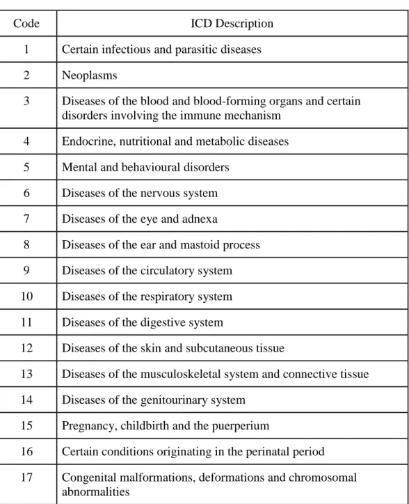
residence to work, service time, age, workload average day, hit target, disciplinary failure, education, son, social drinker, social smoker, pet, weight, height, body mass index. The diseases for absence are attested by the International Code of Diseases (ICD) into 21 categories. The International Classification of Diseases (ICD) is the international "standard diagnostic tool for epidemiology, health management and clinical purposes (International Code of Diseases, para. 1-4).” The ICD of 21 categories are given in the following table--
Table 3.1: Reason for absence with ICD
Code ICD Description
1 Certain infectious and parasitic diseases 2 Neoplasms
3 Diseases of the blood and blood-forming organs and certain disorders involving the immune mechanism
4 Endocrine, nutritional and metabolic diseases 5 Mental and behavioural disorders
6 Diseases of the nervous system 7 Diseases of the eye and adnexa
8 Diseases of the ear and mastoid process 9 Diseases of the circulatory system 10 Diseases of the respiratory system 11 Diseases of the digestive system
12 Diseases of the skin and subcutaneous tissue
13 Diseases of the musculoskeletal system and connective tissue 14 Diseases of the genitourinary system
15 Pregnancy, childbirth and the puerperium
16 Certain conditions originating in the perinatal period 17 Congenital malformations, deformations and chromosomal
abnormalities
18 Symptoms, signs and abnormal clinical and laboratory findings, not elsewhere classified
19 Injury, poisoning and certain other consequences of external causes
20 External causes of morbidity and mortality
21 Factors influencing health status and contact with health services.
There are 7 other categories of reasons for absence as well which are not attested by the ICD given in the table below.
Table 3.2: Reason for absence without ICD
Code Description
22 patient follow up
23 medical consultation
24 blood donation
25 laboratory examination
26 unjustified absence
27 physiotherapy
28 dental consultation
Disciplinary failure, social drinker and social smoker have been encoded from “Yes”
and “No” into “1” and “0” respectively. However, “Education” and “Day of the Week”
have longer categorization which are given in the following tables-- Table 3.3: Code of Day of the week
Code Description
2 Monday
3 Tuesday
4 Wednesday
5 Thursday
6 Saturday
Table 3.4: Code of Education
Code Education
1 High School
2 Graduate
3 Post Graduate
4 Doctorate
In the dataset, only 10 attributes are categorical while the rest of the attributes are numerical. It should be mentioned that there are no missing values in the dataset. The outcome variable in this dataset is named as “absenteeism time in hours” which contains the amount of absenteeism time in hours. However, to make the dataset usable for a classification task, we have transformed the absenteeism time in hours to four classes namely hours, days, weeks and not absent in the new column named “absent_class”.
We found the average time of absent is about 6 hours.
3.3 Data Preprocessing
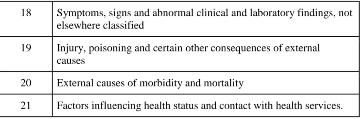
Data preprocessing is one of the most important phases in Machine Learning in order to obtain precise results. The dataset we have collected from the UCI Machine Learning Repository was mostly structured and organized with no missing values. However, we found the values of the output attribute, “absenteeism time in hours” was very dispersed which would be arduous and complicated to obtain good prediction results. We came to a solution of transforming the problem into a classification task to accelerate the prediction results in a more convenient way. We transformed the actual outcome attribute titled “absenteeism time in hours” into a categorical column that includes four classes such that “NOT ABSENT,” “HOURS”, “DAYS”, and “WEEKS” which represents a corresponding amount of time for each class. We have performed this
categorization based on the International Labor Standards on Working Time by International Labor Organization (ILO) (C047-Forty-Hour Week, article section 1, para.1). We have followed the C047 - Forty-Hour Week Convention, 1935 (No. 47) which demonstrates the regulation of working 8 hours a day or 40 hours a week. The set of rules that we have used for transforming the absenteeism hours in absenteeism class is demonstrated in the following table 3.5.
Table 3.5: Classification Rules for the Absenteeism-Time Class of the Dataset Absenteeism Time (x) Absenteeism Class
0 NOT ABSENT
0<x<8 HOURS
40>x>=8 DAYS
x>=40 WEEKS
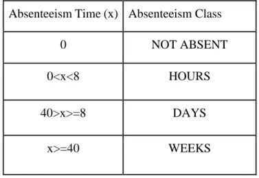
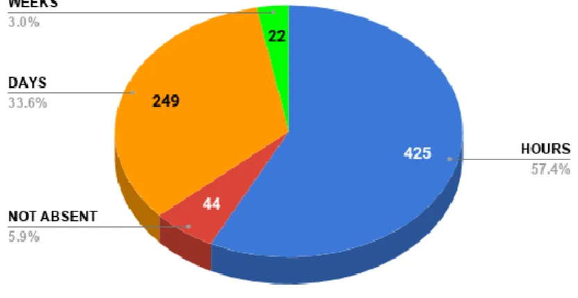
After transforming the hours into class, the dataset contained 5.9% NOT ABSENT, 57.4% HOURS, 33.6% DAYS, and 3.0% WEEKS class. The following Figure 1 shows the class distribution after applying the rules.
Figure 3.2: Class Distribution after Applying the Classification Rules
In the final step, we have omitted the attribute “id” from the dataset as it plays no significant role in the prediction of absenteeism. After performing all the preprocessing steps we finally have 20 features to work on training the machine learning models.
3.4 Partitioning
Data partitioning is basically dividing the dataset into two parts-- training set for using to create machine learning models and learn from the data, and test set to test the actual data with the predicted results. Data partitioning in machine learning acts crucially in order to train better the data and eventually maximize the potential prediction accuracy.
One of the best approaches of data splitting is keeping the train set split ratio as least as possible while ensuring the best prediction model to satisfy the test data that give the highest accuracy. It absolutely varies from dataset to dataset in order to choose the better train and test data ratio. But mostly, 80:20 acts as a rule of thumb method among the practitioners while splitting the dataset (Korjus, 2016). Additionally, all the previous researches based on this absenteeism dataset kept the data splitting ratio as 80:20 (Gayathri, 2018., Martiniano, 2012., Ferraira, 2018.) during the experiment. As
following the early research, we kept the relative ratio for the training set as 80% or 592 instances out of 741 total instances. The remaining 20% instances were kept for the testing part which was 148 instances.
As we were aware of the importance of choosing the right sampling method to achieve the best possible performance, we were convinced to use the random sampling method among the other methods namely Linear Sampling, Take from top, Take from bottom, and Stratified. The linear sampling method always includes the first and the last row and selects the remaining rows linearly over the whole table. This is useful to downsample a sorted column while maintaining minimum and maximum value. Take from top puts the top-most rows into the first output table as the train set and the remainder in the second table as the test set. Similarly, take from the bottom gets the bottom-most rows into the first output table as the train set and the remaining top-most rows as the test set. The stratified sampling method retains the distribution values of the selected column into the output table respectively. As we chose to split the dataset randomly, it helped in resulting with an increased accuracy rate in the predictive model of absenteeism at work. We used a static random seed as 1234 because it helps get reproducible results upon re-execution and to avoid allowing to take a new random seed in each re-execution which might have ended with different outputs in each execution.
3.5 Classification
In machine learning, the technique of predicting the class of a set of given data points is classification. The classes are often called targets or labels. And the given data points are called as features (Machine Learning Classifiers, para.1-4). During the training phase, whether we give both features and actual labels of those features in order to train a machine learning model or to give just the features without letting know the actual
labels. It is because of the different learning techniques as we called supervised or unsupervised. The classifiers we used in this research are the type of supervised machine learning.
We have used a total of three prominent tree-based machine learning techniques for the classification purpose in this study. We have realized that tree-based classifiers can provide a highly effective structure in order to lay out options and investigate the possible outcomes of choosing those options. To form a balanced picture of risks and rewards, the tree based learners also play a significant role. It is easier to interpret to non-technical personnel as tree-based classifiers perform with simple conditional basis.
All the techniques namely Decision Tree, Gradient Boosted Tree, and Random Forest are described in the following subsections.
3.5.1 Decision Tree
In supervised machine learning and data mining, decision tree is one of the most widely used practical methods for inductive interference over the data which are supervised.
The notable feature of decision tree algorithm is constructing the tree without requiring the domain knowledge or parameter setting and yet performing efficiently in exploratory knowledge discovery with the procedure of classifying categorical data based on their attributes (Pal, 2003, p.554-565). The decision tree model is not only simple to understand but also very easy to interpret to others as it comes handy using the feature of displaying trees graphically. As other techniques normally are focused on those datasets that have only one type of variable, decision tree performs better in handling both numerical and categorical data (Gareth, 2015, p. 315). Rather than other approaches, decision trees are more successful in modeling human decisions and behaviors as it is able to mirror decision making more closely (Gareth, 2015).
Decision tree algorithm observes the whole data points and makes a predictive model to predict a particular item’s target value. It creates a one single tree analyzing the relational rules out of the given features and labels. The topmost nodes of that tree play a significant role in a specific prediction problem. To come up with the most suitable and optimized tree it requires to take the correct root node first. It gets help in choosing the right root node by calculating the value Impurity Gini or the Information Gain which are being called as metrics of Decision Tree algorithm. Gini Impurity measures the probability of the incorrect labels from randomly chosen elements or features. By summing up the probability Pi of an item with label i the gini impurity can be calculated.
For a single label the probability would be kiPk = 1-Pi (Decision Tree Learning Wikipedia, para. 1-5). But to compute for a set of items with J classes the following equation is being used--
𝐼𝑔(𝑃) = 1 − ∑ 𝑃𝑖2… … … (3.1)
𝐽
𝑖=1
Information gain often called entropy is used when to concern about making the tree as small and optimized as possible in order to avoid anomalies and over or under-fitting of a tree model. At each node it decides the right features needed to be splitted. Whether a new instance will be classified into yes or no depends the information value which represents the expected amount of information that are required to specify (Witten, 2011, p. 102-103). The equation of entropy is given below.
𝐻(𝑇) = 𝐼𝐸(𝑝1, 𝑝2… … 𝑝𝑗) = − ∑ 𝑝𝑖𝑙𝑜𝑔2𝑝𝑖… … … (3.2)
𝐽
𝑖=1
During the experiment, we carefully considered the important parameters that led us to improvement in generalization performance and, thus, the prediction quality.
Though there are mandatory and optional parameters including class weight, splitting criteria, maximum depth of the tree, maximum features, maximum leaf nodes,
minimum impurity decrease, minimum impurity split, minimum samples leaf, minimum sample spit, minimum weight fraction leaf, splitter, and random state, we kept the parameters as default for this tree except the random state, maximum leaf nodes, and the splitting criteria.
We set random state as 1 to avoid getting different results in re-execution. Maximum leaf nodes allow setting the maximum number of leaves a tree should generate. It is helpful to make the model as small as possible while producing the maximum accuracy score out of a particular dataset. After scrutinizing several times, we
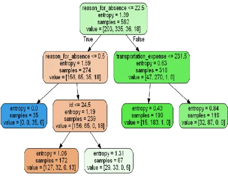
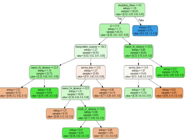
discovered that it produces the maximum score when we set the maximum leaf nodes as 5. And we also followed the entropy techniques to calculate and decide how the features should be split. It yields the following model after fitting with those parameters in our dataset.
Figure 3.3: Decision Tree Model after Fitting the Dataset
3.5.2 Gradient Boosted Tree
Gradient Boosted tree is a first order iterative optimization algorithm which identifies the minimum value of a function. To build an ensemble of trees it uses shallow regression trees and a special form of boosting. In an iterative fashion gradient boosting combines weak “learners” into a single strong learner like other boosting methods (Jenson, 2007, p. 125-139). In each stage, it introduces a weak learner to compensate the shortcomings of existing weak learners. Gradient Boosted Tree tries to find the most optimal tree using the gradient descent reduce loss function. It calculates the loss of each predicted label from the actual label. To find out the gradient of a function with respect to a particular variable it simply does a first order derivation of a function.
Because the first-order derivation projects whether the function increasing or decreasing in order to find out the minimum value. The gradient descent equation is given below—
𝑋𝑛+1 = 𝑋𝑛 − 𝛾. ∆F(𝑋𝑛) … … … . . (3.3)
Here, 𝛾 represents the learning rate such as increment unit which we need to set ensuring it does not exceed the minimum value. The parameters should be considered includes loss function, learning rate, esmitators, subsample, splitting criterion, minimum sample split, minimum samples leaf, minimum weight fraction leaf, maximum depth of trees, minimum impurity decrease, minimum impurity split, random state, maximum features, maximum leaf nodes, etc. After examining several times, we found that maximum leaf nodes should be set 12 in order to get maximum output. We used the default deviance loss function to classify with probabilistic outputs.
We discovered that the learning rate acts as a crucial role for better prediction result.
We set the learning rate as 0.01 while keeping the random state as 1. The measurement
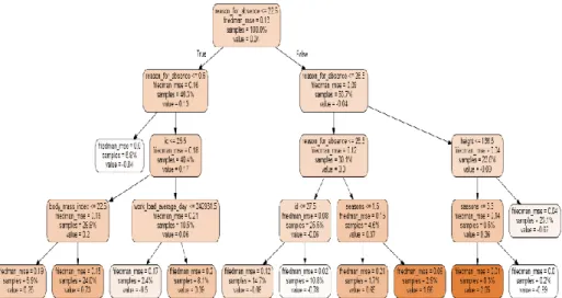
of quality split known as criterion had been set the default Friedman’s Mean Square Error(mse). The number of boosting stage to perform as estimators were set 100. Since Gradient Boosted Algorithm does not work on a single tree, rather perform multiples tree, it only can be visualized the model for different estimators. It is not feasible to showcase the 100 of models which may have slight differences in each tree, but we can project two models for different tree samples of 5 and 42 randomly. The models for tree samples 15 and 73 are given below.
Figure 3.4: Gradient Boosted Tree Model (15) after Fitting the Dataset
Figure 3.5: Gradient Boosted Tree Model (73) after Fitting the Dataset
3.5.3 Random Forest
Random forest is one of the most popular supervised learning algorithm in machine learning which can be used in both regression and classification problems. During the training time, it constructs a multitude of decision trees where each of the decision tree models is learned based on a different set of records and attributes. Precisely it picks the best predictive solution among the decision trees that have been created on randomly selected data samples. In random forest, it, too, decide the root node using the impurity gain and entropy. Unlike Decision tree, it creates over a bunch of decision trees by taking data points randomly. Usually, a very deep grown-up tree tend to learn irrelevant patterns often which causes overfitting or underfitting problem. In that case, decision tree aims to reduce variance by getting trained various parts of the same dataset, and eventually average all the different prediction result in order to improve the overall output. Bootstrap aggregating, also known as bagging, is usually used as the general technique during training in random forest (Moore, 2017). Let, training set, 𝑋 = 𝑥1, 𝑥2… . . 𝑥𝑛 with responses 𝑌 = 𝑦1, 𝑦2, . . . . 𝑦𝑛 and the random sample of training set getting selected repeatedly by baggins as B times. For 𝑏 = 1 … . 𝐵 Averaging the prediction for all individual trees 𝑥’—
𝑓̂ = 1
𝐵 ∑ 𝑓𝑏(𝑥′) … … … (3.4)
𝐵
𝑏=1
The random forest classifier takes the parameter includes estimators as the number of trees in the forest, splitting criteria, maximum depth, min samples split, minimum sample leaf, minimum weight fraction leaf, maximum feature, maximum leaf nodes, minimum impurity decrease, minimum impurity split, bootstrap, random state, class weight, etc.
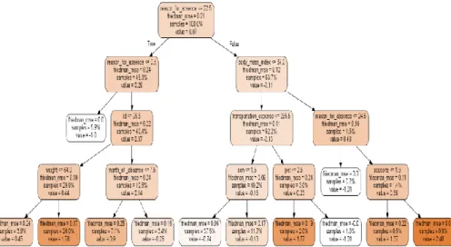
During the experiment, random state was set to 1 as making it same for all classifiers we used in this research. In this model, the maximum leaf nodes as 10 produced the highest prediction accuracy while keeping the split criteria as entropy. Hence it is able to not suffering from the problem of overfitting. We allowed a maximum of 10 models in trees while using the default parameter setting for the remaining parameter.
Likewise, gradient boosted tree it generates multiple trees, so the following tree models are for estimator 1, and 9 respectively.
Figure 3.6: Random Forest Model (1) after Fitting the Dataset
Figure 3.7: Random Forest Model (9) after Fitting the Dataset
So we can see that how randomly random forest picks the potential feature as root nodes in order to reduce or overfitting problem. We also discovered if we extend the maximum tree models then it starts falling down the overall accuracy rate, that’s why maximum-leaf-nodes as 10 is the perfect number in order to get the highest accuracy.
3.6 Summary of this Chapter
After data collection, we classified the absenteeism time into four classes namely NOT ABSENT, HOURS, DAYS, and WEEKS. We splitted the dataset into train and test keeping the ratio as 80:20 while selecting random splitting method. Taking all the features into account we ran three machine learning classifiers namely Decision Tree, Gradient Boosted Tree, and Random Forest.
CHAPTER 4
RESULTS AND DISCUSSION
This chapter is categorized in two following main sections titled Evaluation and Analysis respectively. In the evaluation section, we discussed the metrics that we used to evaluate the model performance of different classifiers. And in the analysis section, we discussed the overall performance of those classifiers.
4.1 Evaluation
In machine learning, there are many ways and metrics in order to evaluate the performance of algorithms. We had to avoid some metrics such as F1 Score and Precision out of the rule of thumb method for evaluating performance, as some classes in different algorithms do not yield F1 Score and Precision. We have used the following seven evaluation metrics (Sokolova, 2009, p. 427-437) to evaluate the performance of the models.
1. Number of True Positives (TP) 2. Number of True Negatives (TN) 3. Number of False Positives (FP) 4. Number of False Negatives (FN) 5. Sensitivity
6. Specificity 7. Accuracy
In machine learning, true positive is the output of a model that yields the correct prediction of the positive class of the target. Likewise, true negative is the outcome of correctly predicting the negative class. The outcome of predicting the positive class of a model incorrectly is called False Positive whereas predicting the negative class
incorrectly is the False Negative. True Positive, True Negative, False Positive, False Negative all these metrics help to understand the statistical comparison of each label that is predicted correctly or incorrectly. A minor improvement can lead to making the best of a particular problem. We used the confusion matrix to derive the value of these TP, FP, TN, and FN for each algorithm. Confusion matrix is also known as Error matrix, which projects the performance of a machine learning algorithm.
Sensitivity, also known as recall, is basically the true positive rate of a model that represents the ability of correctly predicting the true labels. For example, the ability to correctly predicting the Hours, Days, and Weeks classes in our dataset. The following equation is being used for calculating the sensitivity score.
𝑆𝑒𝑛𝑠𝑖𝑡𝑖𝑣𝑖𝑡𝑦 = 𝑇𝑃
𝑇𝑃+𝐹𝑁… … … . (3.5)
Similarly specificity is the proportion of actual negatives that have been predicted correctly. Using the following equation the specificity can be measured—
𝑆𝑝𝑒𝑐𝑖𝑓𝑖𝑐𝑖𝑡𝑦 = 𝑇𝑁
𝑇𝑁+𝐹𝑃… … … . (3.6)
Accuracy score predicts the overall accuracy of a model representing how better the model is. The higher accuracy score represents the better model. It is the ultimate metrics to choose the best classifier who produce the maximum prediction result in our experiment. To calculate the accuracy we need consider the following equation—
𝐴𝑐𝑐𝑢𝑟𝑎𝑐𝑦 = 𝑇𝑃+𝑇𝑁
𝑇𝑃+𝑇𝑁+𝐹𝑃+𝐹𝑁… … … . (3.7)
4.2 Analysis
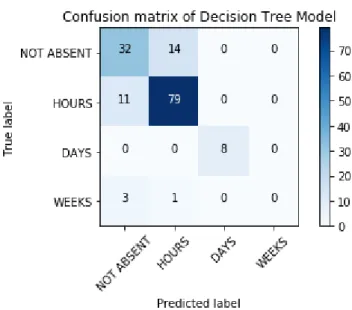
The experimental results are conferred in two dimensions. Firstly, the overall experimental results of all 3 different machine learning algorithms. Secondly, we have demonstrated a comparative analysis of these tree-based machine learning algorithm to discover the impact of each algorithm in the prediction of absenteeism and the algorithm which performs better. Before heading to the first phase, we will first analyze the confusion matrices of these 3 classifiers and derive the value of True Positive, True Negative, False Positive and False Negative for each algorithm. The following figure is the confusion matrix of Decision Tree model.
Figure 4.1: Confusion Matrix of Decision Tree Model
From the confusion matrix of Decision Tree model we can derive the True Positives for four classes as 32, 79, 8, 0 and True Negatives as 88, 43, 140, 144. For the WEEKS class both the True Positive and False Positive are 0.
Figure 4.2: Confusion Matrix of Gradient Boosted Tree Model
From the confusion matrix of Gradient Boosted model we can see a slight increment of True Positives for the NOT ABSENT and WEEKS class, and True Negatives for NOT ABSENT and HOURS Class respectively.
Figure 4.3: Confusion Matrix of Random Forest Model
From Random Forest model we can see that it performs a bit less to predict the NOT ABSENT and HOURS class correctly. However, it performs better in False Negative for NOT ABSENT Class than Decision Tree Model. So now we have to look at the overall measures of all metrics to identify the best classifier. The following table 1 presents the results of those three learning algorithms which reflects the research question number 1 mentioned in the Introduction chapter.
Table 4.1: Evaluation Metrics’ Scores of Different Algorithms True
Positive
False Positive
True Negative
False
Negative Sensitivity Specificity Accuracy
Decision Tree
Not
Absent 32 14 88 14 0.70 0.86
80.41
Hours 79 14 43 11 0.88 0.75
Days 8 0 140 0 1 1
Weeks 0 0 144 4 0 1
Gradient Boosted
Tree Not
Absent 37 13 89 9 0.80 0.87
84.46
Hours 79 10 48 11 0.88 0.82
Days 8 0 140 0 1 1
Weeks 1 0 144 3 0.25 1
Random Forest
Not
Absent 36 14 88 10 0.78 0.86
82.43
Hours 78 12 46 12 0.87 0.80
Days 8 0 140 0 1 1
Weeks 0 0 144 4 0 1
From table 4.1 we can see that Decision Tree identifies all the employees correctly who will be absent at work in daily basis as the True Positive Rate or Sensitivity is 100%
for the “DAYS” class. We can also see that the True Negative rate or Specificity for
“DAYS” and “WEEKS” are 100%. It is able to classify the “HOURS” class correctly as highest as 88%. It completely fails to identify the employees who will be absent in weeks however it is successful in identifying the people who will not be absent in weeks as the specificity is 100%.
In Gradient Boosted Tree, we can clearly see that it improves 25% in the prediction of people who will be absent in weeks while there is no change for the people who will and not will be absent as “DAYS” at all as both sensitivity and specificity are in the maximum. It slightly improves the True Negative Rate for “HOURS” and “DAYS”
from 86% to 87% and 75% to 82% respectively in the comparison of between Decision Tree and Gradient Boosted Tree, meanwhile, a 10% increment in the True Positive Rate for “NOT ABSENT” class.
In Random Forest, we find that it performs better than Decision Tree in predicting
“NOT ABSENT” class as the True Positive Rate is 8% higher. It also improves in True Negative Rate for the “HOURS” class. But there are no changes for “DAYS” and
“WEEKS” in both Decision Tree and Random Forest classifiers.
From a sense of comparative analysis, we understand that all the 3 algorithms yield the maximum possible of sensitivity and specificity score for “DAYS” class as 1.0. For the
“WEEKS” class they also yield the similar sensitivity and specificity score except for the Gradient Boosted Tree algorithm, in which it improves. We find the key differences of scores in the “HOURS” and “NOT ABSENT” class in each algorithm. And that’s a key fact that actually made some algorithm perform better while others do less.
In Decision Tree algorithm it uses just a single optimized tree to predict the target label.
But the scenario is different in Random Forest and Gradient Boosted Tree. Random
Forest instead creates multiple trees taking the root node randomly, and take the average result of the predicted results generated from each tree. That is why Random Forest improves the overall result in some circumstances whereas Decision Tree performs less.
On the other hand, Gradient Boosting itself a type of gradient descent. In each round, it computes the gradient such as the direction in which the model can perform better. And thus it performs better than Random Forest.
Figure 4.4: Accuracy Score of Different Classifiers
From figure 4.4, we can clearly see that the Decision Tree, Gradient Boosted Tree, and Random Forest provides the overall accuracy score as 0.8041, 0.8446, and 0.8243 respectively. The Decision Tree algorithm provides the lowest accuracy rate of 80.41%
while the Gradient Boosted Tree gives the highest accuracy rate of 84.46%.
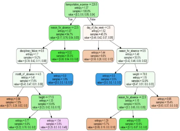
Now to represent the research question 2 mentioned in Chapter 1, we leverage one of the tree-models generated after fitting the dataset into the three learning algorithms.
Since Random Forest and Gradient Boosted Tree have no specific tree-model, and Decision Tree has the only one optimized and root model amongst the other two, we
have to find out the facts using the tree-model generated by Decision Tree algorithm.
The following diagram helps us to understand the facts we are looking for.
Figure 4.5: Learning Model after Fitting the Dataset into Decision Tree Classifier
In a tree model the root node holds the maximum impact of the whole tree because the root node is calculated based on information gain or entropy which defines rationality in order to maximize the final result. From above figure 4.5 we can see that the reason for absence as sickness and the transportation expense are the most vital facts in performing higher absenteeism at workplace.
CHAPTER 5
CONCLUSIONS AND RECOMMENDATIONS
5.1 Findings and Contributions
Absenteeism at work acts as a bottom line in an organization. Employers around the world believe that the absenteeism of employees can have a major effect on company finances, morales and other factors. They do not expect those employees who perform excessive absenteeism at work which cause reducing productivity and thus cost the company.
In this research, our goal was exploring tree-based machine learning algorithms that have never been applied before in this absenteeism dataset. As we applied Decision Tree, Gradient Boosted Tree, and Random Forest in order to predict absenteeism of employees at workplace, we discovered that the tree-based algorithm performs very well. Since there are no such solid researches had taken place after the pioneering research of this dataset, this research firstly represents the application of tree-based learning algorithms by classifying the absenteeism time into four classes according to the International Labor Standards on work time by International Labor Organization (ILO). We found that Decision Tree algorithm provides the lowest accuracy of 80.41%, although it can yield the highest sensitivity score for the “HOURS” class. With the above average score in every evaluation metrics in the prediction of absenteeism of employees at work, the Gradient Boosted Tree classifier produces the highest accuracy of 84.46%.
We also have extracted some insights that the reason for absence as the health and sickness, and the transportation cost from home to work plays a vital role in performing employees’ absenteeism at workplace. And of course, the transportation cost from
home to workplace determines the potential employees who should be considered carefully by organizations. The insights of absenteeism of employees at work could leverage throughout an organization’s both internally and externally. Though it varies from organization to organization, place to place, however, the insights will always be impactful to a company for better monitoring and control of employees. Perhaps it can contribute in the employee recruitment as well through leveraging the insights and patterns.
5.2 Recommendations for Future Works
In our future work, we aim to apply feature engineering on the dataset in order to increase the best possible accuracy score for predicting absenteeism of employees at workplace. Moreover, we intend to extend our work on a real dataset based in Bangladesh. We are in progress with some official processes of collecting employee performance and attendance data of Daffodil International University. We aim to find patterns and insights of employees who perform absenteeism and make a comparison study between Bangladesh and international perspectives. Although employee management research has been taking places since a long ago, however, it is comparatively new in taking a machine learning approach for absenteeism research.
REFERENCES
Altman, DG., & Bland, JM. (1994). Diagnostic tests. 1: Sensitivity and specificity.
BMJ. 308 (6943): 1552. doi:10.1136/bmj.308.6943.1552. PMC 2540489. PMID 8019315.
Anaconda Wikipedia. Retrieved on 27/11/2018, from
https://en.wikipedia.org/wiki/Anaconda_(Python_distribution).
Albion, J, M. et al. (2008). Predicting absenteeism and turnover intentions in the health professions. Australian Health Review Vol 32 No 2
Anaconda Navigator. Retrieved on 2/11/2018, from
https://docs.anaconda.com/anaconda/navigator/
Berg, T, Y., Elders, LA., & Burdorf, A. (2009). The effects of work-related and individual factors on the Work Ability Index: a systematic review. Occup Environ Med 2009;66:211–220
CO47-Fourty-hour week convention. Retrieved on 27/11/2018, from https://www.ilo.org/dyn/normlex/en/f?p=NORMLEXPUB:12100:0::NO::P12100_IL O_CODE:C047.
Decision Tree Learning Wikipedia. Retrieved on 28/11/2018, from https://en.wikipedia.org/wiki/Decision_tree_learning#Gini_impurity.
De’ath, G. (2007). Boosted Trees For Ecological Modeling And Prediction. Ecological Society of America, Ecology, 88(1), pp. 243-251
Dietterich, T, G. (2000). Ensemble Methods in Machine Learning. International Workshop on Multiple Classifier Systems, Multiple Classifier Systems pp. 1-15.
Ferreira, R, P. et al. (2018). Artificial Neural Network And Their Application In The Prediction of Absenteeism At Work. Int J Recent Sci Res. 9(1), pp. 23332-23334 Gayathri, T. (2018). Data mining of absentee data to increase productivity. International Journal of Engineering and Techniques - Volume 4 Issue 3, May 2018
Gunnar, B., et al. (2009). Sickness Presenteeism Today, Sickness Absenteeism Tomorrow? A Prospective Study on Sickness Presenteeism and Future Sickness Absenteeism. Journal of Occupational and Environmental Medicine, 51(6), pp. 629- 638.
Gareth, J. et al. (2015). An Introduction to Statistical Learning. New York: Springer. p.
315. ISBN 978-1-4614-7137-0.
Gangai, K, N. (2014). Absenteeism at workplace: what are the factors influencing it?, Volume 3, ISSN: 2279-0950.
Galiano, R, V, F. et al. (2012). An assessment of the effectiveness of a random forest classifier for land-cover classification.
Hastie, T., Tibshirani, R., & Friedman, J. (2008). The Elements of Statistical Learning (2nd ed.). Springer. ISBN 0-387-95284-5.
Jenson, S., & McIntosh, J. (2007). Absenteeism in the workplace: results from Danish sample survey data, Empirical Economics, Volume 32, Issue 1, pp. 125-139
Johns, G. (2010). Presenteeism in the workplace: A review and research agenda.
Journal of Organizational Behavior. vol. 31, p. 519 – 542,2010.
Jupyter Notebook Wikipedia. Retrieved on 27/11/2018 from https://en.wikipedia.org/wiki/Project_Jupyter.
Korjus, K., Hebart, M, N., & Vicente, R. (2016). An Efficient Data Partitioning to Improve Classification Performance While Keeping Parameters Interpretable. DOI:
10.1371/journal .pone . 0161788
Martiniano, A., Ferreira, R. P., Sassi, R. J., & Affonso, C. (2012). Application of a neuro fuzzy network in prediction of absenteeism at work. In Information Systems and Technologies (CISTI), 7th Iberian Conference on (pp. 1-4).
Machine Learning Classifiers. Retrieved on 28/11/2018, from https://towardsdatascience.com/machine-learning-classifiers-a5cc4e1b0623.
Martiniano, A., Ferreira, R. P., & Sassi, R. J. (2018). UCI Machine Learning Repository [https://archive.ics.uci.edu/ml/datasets/Absenteeism+at+work]. Sao Paulo, Brazil:
Universidade Nove de Julho - Postgraduate Program in Informatics and Knowledge Management.
Moore, A., Cai, Y., Jones, K., Murdock, V. (2017). Tree Ensemble Explainability.
International Conference on Machine Learning, Sydney, Australia, PMLR 70, 2017.
Numpy Wikipedia. Retrieved on 27/11/2018, from
https://en.wikipedia.org/wiki/NumPy.
Nunung, N., Qomariyah, Y, G., Sucahyo. (2014). Employees’ attendance patterns prediction using classification algorithm case study: a private company in Indonesia.
Int’l Journal of Computing, Communications & Instrumentation Engg.(IJCCIE) Vol. 1, Issue 1(2014) ISSN 2349-1469 EISSN 2349-1477.
Pandas Wikipedia. Retrieved on 27/11/2018, from
https://en.wikipedia.org/wiki/Pandas_(software)
Pal, M., & Mather, P, M. (2003). An assessment of the effectiveness of decision tree methods for land cover classification. Remote Sensing of Environment 86(2003) .pp.
554-565, ScienceDirect.
Python for Artificial Intelligence. Retrieved on 27/11/2018, from https://en.wikipedia.org/wiki/Scikit-learn]. Retrieved on 27/11/2018.
Python Plotting. Retrieved on 27/11/2018, from https://matplotlib.org/
Schouteten, R. (2017). Predicting absenteeism: screening for work ability or burnout.
Advance Access publication Occupational Medicine 2017;67:52–57
Silva, A, M., Ferreira, R, P., & Sassi, R, J. (2010). Control and monitoring of the indexes of absenteeism and presenteeism with aid of the technology of the information.
CONTECSI - 2010, ISBN: 978-85-99693-06-3, 2010.
Silva, L, S., et al.(2011). do absenteísmo em um banco estatal em Minas Gerais: análise no período de 1998 a 2003. Acessado em: 20 de jan. 2011.
Sokolova, M., & Lapalme, G. (2009). A systematic analysis of performance measures for classification tasks. Information Processing and Management 45 (2009) 427–437 Smyth, PS, F. (1996). "From Data Mining to Knowledge Discovery: An Overview".
Advances in Knowledge Discovery and Data Mining, AAAI Press / The MIT Press, Menlo Park, CA, 1996, pp.1-34
The Causes and Costs of Absenteeism. Retrieved on 28/11/2018, from https://www.forbes.com/sites/investopedia/2013/07/10/the-causes-and-costs-of-
absenteeism-in-the-workplace/#175d79ef3eb6.
Witten, I., Frank, E., & Hall, M. (2011). Data Mining. Burlington, MA: Morgan Kaufmann. pp. 102–103. ISBN 978-0-12-374856-0.
WHO, International Code of Diseases. Retrieved on 27/11/2018, from http://www.who.int/classifications/icd/en/
Appendix – A
Parameters of Absenteeism at Work Data Set
Full Name Column Name Type Value
Individual Identification
id Number
Reason for Absence
reason_for_absence Certain
infectious and parasitic diseases ; Neoplasms;
Diseases of the blood and blood-
forming organs and certain
disorders involving the
immune mechanism;
Endocrine, nutritional and
metabolic diseases;
Mental and behavioural disorders ; Diseases of the nervous system ;
Diseases of the eye and adnexa ;
Diseases of the ear and mastoid
process ; Diseases of the
circulatory system;
Diseases of the respiratory
system;
1
2
3
4
5
6 7 8
9 10 11 12
Diseases of the digestive
system;
Diseases of the skin and subcutaneous
tissue ; Diseases of the musculoskeletal
system and connective
tissue;
Diseases of the genitourinary
system;
Pregnancy, childbirth and the puerperium ;
Certain conditions originating in
the perinatal period ; Congenital malformations,
deformations and chromosomal abnormalities ; Symptoms, signs
and abnormal clinical and
laboratory findings, not
elsewhere classified ;
Injury, poisoning and
certain other consequences of external causes ;
13
14
15
16
17
18
19
20
21 22
External causes of morbidity and
mortality;
Factors influencing health status and
contact with health services.;
patient follow- up;
medical consultation;
blood donation;
laboratory examination;
unjustified absence;
physiotherapy;
dental
consultation 23 24 25 26 27 28
Month of Absence month_of_absence January
February March
April May June
July August September
October November December
1 2 3 4 5 6 7 8 9 10 11 12
Day of the Week day_of_the_week Monday
Tuesday Wednesday
Thursday Friday
2 3 4 5 6
Seasons seasons Spring
Summer Fall Autumn
1 2 3 4