A PRIVACY-ENHANCED APPROACH FOR PLANNING SAFE ROUTES WITH CROWDSOURCED DATA AND

(1)

M.Sc. Engg. (CSE) Thesis

A PRIVACY-ENHANCED APPROACH FOR PLANNING SAFE ROUTES WITH CROWDSOURCED DATA AND

COMPUTATION

Submitted by

Fariha Tabassum Islam 1018052029

Supervised by

Dr. Tanzima Hashem

Submitted to

Department of Computer Science and Engineering Bangladesh University of Engineering and Technology

Dhaka, Bangladesh

in partial fulfillment of the requirements for the degree of Master of Science in Computer Science and Engineering

(2)

(3)

(4)

Acknowledgement

Foremost, I am eternally grateful to Allah SWT. the most gracious and the most merciful.

I would like to express my sincerest gratitude, deep respect and admiration to my supervisor, Professor Dr. Tanzima Hashem, who taught me how to do research. I have been extremely lucky to have her as my supervisor. I am indebted to her for her constant supervision, clear guidance, great encouragement and motivation and all the efforts she put on me. This thesis would never be completed without her guidance, directions and help in every aspect. She spent numerous valuable hours of her busy schedule addressing the problems I faced promptly and correcting the manuscript. Her immense wisdom and experience have helped me in all the time of my research life.

I am grateful to Dr. Rifat Shahriyar for his guidance and valuable suggestions and for reviewing the draft. I also want to express my gratitude to the members of my thesis committee for their valuable suggestions. I thank Dr. A.K.M. Ashikur Rahman, Dr. A.B.M. Alim Al Islam, Mr. Sukarna Barua, and specially the external member Dr. Mohammad Nurul Huda.

I gratefully acknowledge the fellowship I received from the ICT Division, Bangladesh (56.00.0000.028.33.108.18). I thank the Department of CSE, BUET, for providing resources during the thesis work.

I remain ever grateful to my beloved parents and my beloved husband Tareq who always inspired me and provided unlimited support in every success and failure.

Dhaka Fariha Tabassum Islam

June 28, 2021 1018052029

iii

(5)

List of Figures

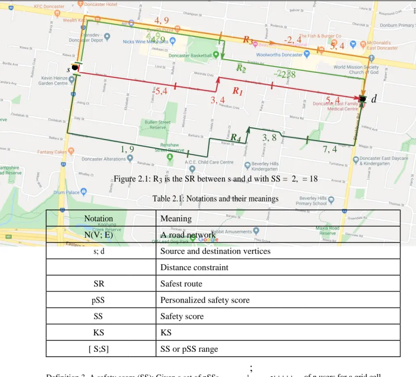
2.1 R3 is the SR between s and d with SS = 2, = 18 . . . 5

3.1 A KD-tree . . . 11

3.2 An point region quadtree . . . 12

3.3 An R-tree . . . 13

4.1 System architecture . . . 16

4.2 A user’s pSSs is stored in a modified R-tree . . . 20

4.3 Necessary MBRs for updating a supercell . . . 21

4.4 A small road network and an SR query for showing the simulations of Dir OA and It OA ... 27

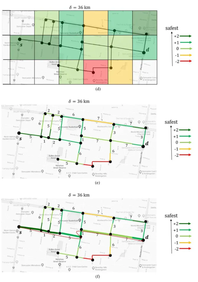
4.5 Simulation of Dir OA... 28

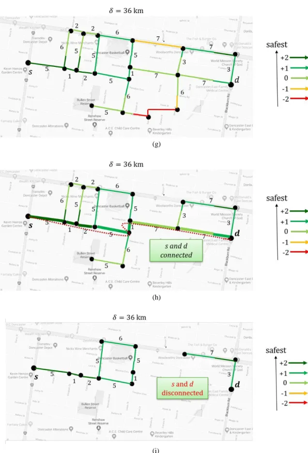
4.6 Simulation of Dir OA (continued) . . . 33

4.7 Simulation of It OA... 40

4.8 Simulation of Xit . . . 42

5.1 Choosing default value Xit = 50 based on the effects of X_it . . . 48

5.2 Dir OA vs. It OA in terms of privacy (#pSSs revealed) and computation cost (comm. freq. and runtime) for varying , d_q and d_G . . . 49

5.3 Accuracy loss in the centralized model for missing data. C50 means 50% of actual data is present. . . . 51

5.4 Confidence level for our system is higher than that of the centralized model (Chicago dataset). . . 53

5.5 Confidence level for our system is higher than that of the centralized model (Beijing dataset). . . . 54

5.6 Confidence level for our system is higher than that of the centralized model (Philadelphia dataset). . . 55

vi

(8)

List of Tables

2.1 Notations and their meanings . . . 5

3.1 A comparative analysis with existing safe route planners . . . 8

5.1 Datasets . . . 45

5.2 Parameter settings . . . 47

5.3 The percentage of query samples for which top-K shortest routes include the respective SRs . . . 56

5.4 The actual distance constraint ratio of the lengths between the SR and the shortest route . . . 56

vii

(9)

Abstract

In this thesis, we introduce a novel safe route planning problem and develop an efficient solution to ensure the travelers’ safety on roads. Though few research attempts have been made in this regard, all of them assume that people share their sensitive travel experiences with a centralized entity for finding the safest routes, which is not ideal in practice for privacy reasons. As a result, existing systems cannot provide safest routes with high accuracy due to the lack of data related to travel experiences. Furthermore, existing works formulate the safe route planning query in ways that do not meet a traveler’s need for safe travel on roads. Our approach finds the safest routes within a user-specified distance threshold based on the personalized travel experience of the knowledgeable crowd without involving any centralized computation. We develop a privacy preserving model to quantify the travel experience of a user into personalized safety scores. Our algorithms for finding the safest route further enhance user privacy by minimizing the exposure of personalized safety scores with others.

Specifically, we develop two efficient algorithms, direct and iterative, to evaluate the safest route queries. The direct and the iterative algorithms offer trade-offs among the computation overhead, communication cost and privacy. We run extensive experiments using three real datasets to show the effectiveness and efficiency of our approach. Our iterative algorithm finds the safest route with 50% less exposure of personalized safety scores compared to that of direct algorithm. On the other hand, the computation overhead and the communication overhead for the direct algorithm are lower compared to those of the iterative algorithm.

Although the direct algorithm is faster than the iterative algorithm, both of our algorithms take less than a second to process a query. Our experiments also show that lack of data for privacy issues can reduce the answer quality significantly. Our safe route planning system ensures the quality of the safest routes by protecting the privacy of the travel experiences of the users.

viii

(10)

Chapter 1 Introduction

Location-based services, especially the journey planners like Google or Bing Maps, have become an integral part of our life for moving on roads with convenience. Existing services mainly consider distance and traffic while planning the routes for the travelers. However, the shortest or the fastest route is not always the best choice. While travelling on roads, people face many inconveniences like theft and pick- pocketing; women face harassment like eve-teasing and unwanted physical touch. People would like to travel a little bit longer on a safer route that avoids those inconveniences. During the outbreak of an infectious disease like COVID-19, a pedestrian may want to avoid a crowded road to keep herself safe from infection. The chance for a virus to exist on the air and road surface increases with the increase of the number of pedestrians. Road safety in such a pandemic period can be measured based on the level of road crowdedness. To meet the traveler’s need on roads, we introduce a safe route planner that finds the safest route (SR) between a source-destination pair within a distance constraint.

The data needed for computing the SRs may come from official crime reports and personal travel experiences of the crowd. The latter is more valuable than the former one due to its recency and adequacy. However, travel experiences are often sensitive and private data, and people, especially women, do not feel comfortable sharing their detailed travel experiences and harassment data with others [1]. These factors have inspired us to develop a privacy- enhanced safe route planning system by not sharing the personalized travel experiences of the crowd with a centralized entity or others.

Our approach personalizes the safety score (SS) of a user’s travel experience (both safe and unsafe) with respect to the user’s travel pattern. If two users face the same crime on two roads, then these roads may have different SSs considering the frequency and recency of the users’

1

(11)

2

visits on those roads. Ignoring the personal travel pattern of the users would reduce the quality of data and the accuracy of the query answer. We develop a model to quantify a user’s travel experience for a visited area into a personalized safety score (pSS) based on frequency and recency of the user’s visits, location, time, and type of inconveniences faced. Users store their pSSs of their known areas on their own device or any other private storage (e.g., cloud storage) and use them to find the SRs for others. The transformation of a user’s travel experience into a pSS is a one-way mapping. From the revealed pSS of a user, it is not possible to pinpoint the type of incident faced by the user. It may only allow an adversary to infer high- level information on a user’s travel experience (e.g., a user faced a crime event without knowing the crime type).

To further enhance user privacy, we minimize the amount of pSS information shared to evaluate the SR query. We develop efficient query processing algorithms that find the SRs from the refined search space and minimize the exposure of pSS information. Since the number of possible routes between a source- destination pair is extremely high, a naive algorithm cannot find the SRs in real-time. Our search space refinement techniques allow our query processing algorithms to find the SRs with significantly reduced processing overhead.

Every user is not familiar with all roads, and it is also not feasible to involve a user for all queries. For a specific SR query, we identify the users who are familiar with the query-relevant area and select them as group members. The trustworthiness of the query answer depends on the overall knowledge of the selected group members. To show the credibility of the answer, we present a new measure called confidence level [2, 3] in the context of the SR query.

Existing safe route planners involve a centralized entity to find the SRs using crime data collected from reports [4] or crowd [5] or both [6–8]. They have major limitations:

• Ignore the privacy issues of the crowd harassment and incident data and thus suffer from data scarcity problem. Missing incident data can cause a system to return a route that is not actually safe and put a traveler at risk.

• Do not personalize the crowd’s travel experiences by considering a user’s travel pattern, which is essential to improve the accuracy of the query answer.

• Do not consider individual distances associated with different SSs for ranking the routes.

For example, if two routes have the same lowest SS, then the route for which a user has to travel less distance with the lowest SS is the safest one, though its total distance might be greater than that of the other route.

• Do not show any measure to represent the trustworthiness of the identified SRs.

(12)

3

In recent years, the increase of computational power and storage in smartphones has enabled researchers to envision crowdsourced systems [2, 3, 9]. To the best of our knowledge, we propose the first privacy-enhanced and personalized solution for the SR queries with crowdsourced data and computation. Our solution overcomes the limitations of existing route planners. Our contributions are as follows:

• We present a model to quantify a user’s travel experiences into irreversible pSSs and modify the indexing technique, R-tree to store pSSs. Based on pSSs, we design a privacy-enhanced crowd-enabled solution for the SR queries.

• We select the users who have the required knowledge in a query-relevant area, and we guarantee the credibility of the query answer evaluated based on the data of the selected group members in terms of the confidence level.

• We develop optimal algorithms, direct and iterative, to efficiently evaluate the SRs. The direct algorithm reveals group members’ pSSs only for the query-relevant area. The iterative one further reduces the amount of shared pSSs at the cost of multiple communications per group member.

• We run extensive experiments with real datasets and evaluate the effectiveness and efficiency of our approach.

This thesis is organized as follows. First, we formulate our problem in Chapter 2. Then, we discuss previous works related to our problem in Chapter 3. In Chapter 4, we elaborate our safe route planning system by providing an overview of our system, our personalized safety quantification model, our indexing techniques, the algorithms and the privacy-preserving aspects of our work. In Chapter 5, we evaluate the effectiveness and efficiency of our algorithms through extensive experiments. Finally, we conclude our work with future directions in Chapter 6.

(13)

Chapter 2 Problem Formulation

We define basic terminologies and notations, explain the ranking of routes based on safety and formulate our problem for finding the safest route in this chapter. We also describe our privacy model. In Section 2.1, the necessary notations, definitions, and terminologies are given. Then in Section 2.2, we elaborately discuss our privacy model.

2.1 Preliminaries

The road network N = (V; E) consists of a set of vertices V and a set of road segments E. The vertices represent the start or the end or the intersection points of roads. An edge e_ij 2 E connects the vertex v_i to the vertex v_j, where v_i; v_j 2 V . A route R consists of a sequence of vertices R = (v_i1 ; v_i2 ; : : : ; v_ijRj), where e_ik1i^k 2 E. The total distance dist(R) of R is the summation of distances of all edges in R. Table 2.1 shows the notations used in this thesis.

The total space is divided into grid cells. The knowledge score (KS), the pSS and the SS are computed for each grid cell area, which are defined as follows:

Definition 1. A knowledge score (KS): The KS of a user for a grid cell area represents whether the user has visited the area of a grid cell. This KS is 0 if the user has not visited the area in the last w days, 1 otherwise.

Definition 2. A personalized safety score (pSS): Given the safety score bound [ S; S], the pSS of a grid cell area represents a user’s travel experience in the area and is quantified between

S pSS S.

4

(14)

2.1. PRELIMINARIES 5

s

4, 9

4, 9 R₃ -2, 4

5, 4 R₂

-2, 8 R₁

-5,4

3, 4 5, 4

d

1, 9

R₄ 3, 8

7, 4

Figure 2.1: R₃ is the SR between s and d with SS = 2, = 18 Table 2.1: Notations and their meanings

Notation Meaning

N(V; E) A road network

s; d Source and destination vertices Distance constraint

SR Safest route

pSS Personalized safety score

SS Safety score

KS KS

[ S;S] SS or pSS range

Definition 3. A safety score (SS): Given a set of pSSs ¹

;

2; : : : ;

n of n users for a grid cell

area, the SS of the grid cell area is computed as

1+

+:::+ _n

.

2

n

To make the SS measure independent of the number of users who know about an area, we take the average of the pSSs instead of adding them together. The number of users whose pSSs are used to find the SS is considered to determine the credibility of the safest route (Section 5.3.2).

SS based route ranking. The SS of route R is the minimum of all SSs associated with the edges of R. The intuition behind considering the minimum SS instead of the average SS of the route is that even a small distance of road with a bad SS may put a traveler at risk. The route that has the

(15)

2.2. PRIVACY MODEL 6

largest minimum SS among all possible routes between a source-destination pair is considered as the SR. If two routes have the same largest minimum SS, then we consider the smallest SS for which associated distances of two routes differ. The route that has the smallest associated distance for the considered SS, is the SR. We formally define the SR query below:

Definition 4. A safest route (SR) query: Given a road network N(V; E), distances and SSs of road segments, a source location s, a destination location d and a distance constraint , the safest route query returns a route SR between s and d such that dist(SR) and SR is at least as safe as R, where R is any other route between s and d having dist(R) .

In Fig. 2.1, assume that = 18. The distance of R₁, R₂, R₃ and R₄ are 12, 17, 17, 21 respectively.

R₄ does not satisfy . The smallest SSs associated with R₁, R₂ and R₃ are -5, -2 and -2, respectively. Though both R₂ and R₃ have the largest minimum SS, R₃ is the SR because R₃ has the smallest distance associated with the smallest SS -2.

2.2 Privacy model

We assume a semi-honest setting, where participants follow the system protocol but are curious to infer sensitive data from the shared information. In the semi-honest setting, the participants do not send false queries (e.g. unnecessary queries) or wrong pSSs and they do not collude with each other or any centralized entity. In our system, the unsafe event types (e.g., pick-pocketing or harassment) are considered as private data. We assume that anyone can play the role of an adversary for a user. The adversary knows the model to compute the pSSs but does not have any background knowledge about the time and frequency of a user’s visits to an area. A user shares the KSs and pSSs for the purpose of the query evaluation. Our solution refrains an adversary from inferring the unsafe event type that a user encounters from the shared information of the user. Since a pSS can reveal high-level information like a user faced an unsafe event but not the type, our solution also aims to minimize the number of revealed pSSs for enhancing a user’s privacy.

(16)

Chapter 3 Related Works

We address the problem of finding the safest route in a crowdsourced manner in this research.

Therefore, this problem is closely related to the research works on route planning and crowdsourcing. This chapter provides elaborate discussions on existing research works relevant to our thesis. In Section 3.1, we focus on the existing works on the safe route planners. We compare those works with ours based on the problem setting (Section 3.1.1), privacy (Section 3.1.2), and efficiency (Section 3.1.3). In Section 3.2, we discuss the shortest path algorithms, in Section 3.3, we focus on other route planners, and in Section 3.4, we detail various indexing techniques that are used to store data in an organized way. Finally in Section 3.5, we present the existing works on crowdsourcing.

3.1 Safe Route Planners

Though researchers attempted to solve the safe route planning problem, the works have major limitations. Table 3.1 shows the problem settings and other features of existing works.

3.1.1

Problem Setting

None of the existing works considers individual distances associated with different SSs for ranking the routes after maximizing the minimum SS. Thus, the problem settings of existing works are not suitable for safe travel on roads. Furthermore, instead of considering the total

7

(17)

3.1. SAFE ROUTE PLANNERS 8

Table 3.1: A comparative analysis with existing safe route planners

Problem Settings

Privacy Efficiency

Safety

pSS Objective

Level

[4] Multiple Provide multiple routes with a X

trade-off between SS and total

distance

[5] Safe/Unsafe Minimize the travel in unsafe

regions

[6, 7] Multiple Minimize the weighted

combination of SS and total

distance

[10] Safe/Unsafe Minimize the travel in unsafe X

regions

ours Multiple Maximize the minimum SS of X X X

the route and then minimize the

individual distances associated

with the SSs in the increasing

order of SSs

distance constraint, selecting appropriate weights in [6, 7] is not easy since it is not intuitive to determine which weights would meet a user’s preferred trade-off between safety and distance for a specific source-destination pair. Again, there is no guarantee that the returned routes in [4]

satisfy a user’s required preference for safety and distance.

3.1.2 Privacy

The crime data for safe route planners may come from crime reports [4, 8, 11] or directly from crowds [5–8]. Crime reports are not regularly updated, and incomplete because many crimes go unreported. Though the crowd knows more and recent information compared to the crime reports, they would not share their incident and harassment data with a centralized service provider, if the privacy of their data is not ensured. Thus, one major limitation of existing works is that they suffer from data scarcity issues for privacy reasons and do not have enough data to provide accurate answers.

(18)

3.2. SHORTEST PATH ALGORITHMS 9

3.1.3 Efficiency

None of the existing safe route planning systems except [4, 10] developed efficient algorithms for large road networks. However, as already mentioned, the problem settings of [4, 10]

cannot meet a traveler’s requirement on roads.

3.2 Shortest Path Algorithms

Researchers have proposed many algorithms to solve the shortest path problem or its variant [12–18] over the last few decades. Research on this topic is still ongoing [19–21]. The shortest path problems can be divided into three types:

1. All-pair shortest path problem 2. Single-source shortest path problem 3. Single-pair shortest path problem

The all-pair shortest path problem can be solved using Floyd–Warshall algorithm [22], Johnson Algorithm [23]. The single-source shortest path problem can be solved by Dijkstra’s algorithm [12], Bellman-Ford algorithm [24]. The single-pair shortest path can be solved using the algorithms for the single-source shortest path problem. We can also use A* searching [25] for the single-source shortest path problem. Many improvements have been proposed in these core algorithms for finding the shortest path [26, 27]. Many variants [28–33] of the shortest path problem exist, such as the shortest path with constraints [28,29] and multi-objective shortest path problem [30]. Meta-heuristic algorithms have been also applied to solve these problems [34, 35].

Some researchers have maintained privacy while computing the shortest path for navigation [17, 36]. The authors of [18] used the Bellman-Ford algorithm to plan energy-efficient driving routes.

For this research, we have used the single-pair shortest path algorithm to refine the search space in Section 4.4.2. Furthermore, in Section 5, we have defined the distance constraint for an SR query based on the shortest road network distance to simplify its implication to users.

(19)

3.3. OTHER ROUTE PLANNERS 10

3.3 Other Route Planners

Variants of orienteering and scheduling problems [37, 38] have been studied for route planning.

An orienteering problem finds a route between a source-destination pair that maximizes the total score within a budget constraint, where a score is obtained when the route goes through a vertex.

The scheduling problems focus on incorporating temporal constraints in route planning (e.g., visiting locations to perform services in a timely manner). The problem settings of orienteering and scheduling problems are different from an SR query. Furthermore, their solutions do not consider search space refinement [39] and are not scalable for large road networks. For example, the exact solution of an orienteering problem can be found for a graph of up to 500 vertices [38], whereas the real road networks that we use in our experiments have on average 24 thousand vertices.

An SR query can be transformed to a multilevel optimization problem for solving it with a commercial optimization tool like IBM CPLEX: (L1) identify all routes that have the largest minimum SS within , (L2) consider the smallest SS for which the associated length of the identified routes differs and find the routes that have the smallest length associated with the considered SS, (L3) repeat L2 until the remaining route(s) have the same length associated with every SS. However, IBM CPLEX is not effective in terms of time and memory when a problem requires finding multiple answers like multiple routes with the same largest minimum SS in the SR query [40].

3.4 Indexing

We need to store KSs and pSSs in our system. These are spatial data. Indexing techniques for storing spatial data have been studied extensively in the literature [41–43]. Spatial data can be two dimensional or multidimensional. Spatial data includes points, lines, polygons etc. The number of samples can be huge.

We need to store, access and manipulate them efficiently for a variety of applications. Specially, we need to perform range queries in spatial data frequently to access data near or within a particular area. Using a list or map can be costly storage-wise and is not efficient for range queries. Therefore, many indexing techniques for spatial data exploit the tree-based structure to store and access data efficiently. Following we describe some of them.

(20)

3.4. INDEXING 11

3.4.1 KD-tree

The KD-tree [44] is essentially a multidimensional binary search tree that stores multidimensional points. A new point is inserted in a leaf node. Each internal node of the tree divides a particular plane.

For a k dimensional tree, a level l divides the (l mod k)-th plane (if (l mod k) is 0, it divides the kth plane). Figure 3.1 shows an example of a KD-tree. A KD-tree has some limitations because its shape depends on the order of input, and in the worst case, it may contain n levels [42]. Variations of the KD- tree has been proposed to overcome these limitations, such as an adaptive KD-tree [45], KDB-tree [46]. However, these variations also have their limitations; e.g. the adaptive KD-tree is not dynamic.

(a) A KD-tree (b) Plane division by a KD-tree

Figure 3.1: A KD-tree

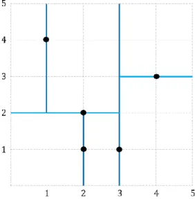
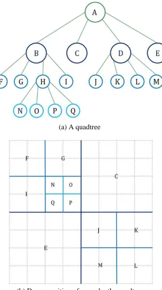
3.4.2

Quadtree

A quadtree recursively decomposes a space into four quadrants. There are different types of quadtree, such as point quadtree, point region quadtree, region quadtree and polygonal map quadtree [42]. The point quadtree is similar to KD-tree, except the fact that each internal node has exactly four children. The point region quadtree is slightly different from the point quadtree. It divides the space into four equal quadrants and does not use the data points for plane decomposition. An example of this type of tree is given in Figure 3.2. A region quadtree generally stores an approximation of a polygon. Finally, a polygon map quadtree is used to store a set of polygons [47].

(21)

3.4. INDEXING 12

(a) A quadtree

(b) Decomposition of space by the quadtree

Figure 3.2: An point region quadtree

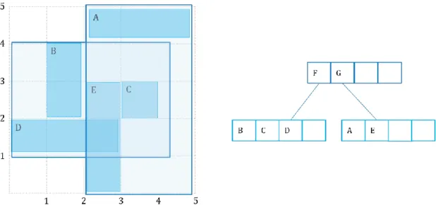
3.4.3 R-tree

An R-tree is a spatial indexing structure proposed in 1984 by Antonin Guttman [48]. Figure 3.3 shows an example of an R-tree that stores rectangles. An R-tree is a multiway tree whose leaf node contains the spatial objects, such as point, line, polygon etc. The internal nodes group nearby objects together using a minimum bounding rectangle (MBR). There is a limit on how many entries each node can have. If that limit is exceeded when inserting data, then that node is split. The R-tree allows the overlap among MBRs of the internals nodes of the same level (e.g. MBR F and G in Figure 3.3) and frequently, the internal nodes cover some empty spaces. Fewer overlaps and empty spaces increase the R-tree’s efficiency.

Multiple variations of the R-tree have been proposed including R+-tree [49], R*-tree [50] and Hilbert R-tree [51]. The R+-tree is an efficient version of the R-tree that avoids the overlap

(22)

3.5. CROWDSOURCING 13

(a) Two-dimensional rectangles (A, B, C, D, E) in (b) An R-tree constructed from those rectangles a plane

Figure 3.3: An R-tree

among MBRs. However, this comes at the price of more nodes and space [42, 43]. Also, the construction and modification are more complex. R+-tree is more efficient for the point query search, however, range queries can be costly [43]. The R*-tree differs from the R-tree in terms of the insertions. When a node becomes overfull while inserting data, instead of splitting that node immediately, some entries are tried to be reinserted in that tree first. The Hilbert R-tree organizes the data based on Hilbert value, which is efficient but might not always be realistic [42].

For storing the pSSs in a user’s personal device, we chose to modify an R-tree because we need to perform the range queries for retrieving pSSs by utilizing the low computational power and low space capacity of mobile devices. Its variants are either too complex or require more space. Instead of using the R-tree directly, we modified it because we wanted to reduce space consumption by keeping the same pSS information of nearby grid cells together.

3.5 Crowdsourcing

Crowdsourcing has been widely used for route finding and recommendation [52–62], trip planning [63–65], POI search [2, 3, 66], POI summarization [67], package delivery [68, 69], sensing [70–72], traffic monitoring [73, 74], vehicular network [75], indoor mapping and localization [76–78] and many other tasks [79].

(23)

3.5. CROWDSOURCING 14

The works in [3,9] eliminate the location-based central service provider to protect users’ sensitive location data and divided the query evaluation task among the selected group. While evaluating a query, those works preserve privacy through data imprecision. In [2], the authors considered protecting the privacy of a user’s POI knowledge by minimizing the shared POI information with others. Compared to the static POI data, crime data are more complex and challenging to hide from others. We develop a quantification model to hide the type of incident data using pSS and search space refinement techniques to minimize the shared pSS information.

(24)

Chapter 4 Our Approach

In this chapter, we explain in detail our approach for finding the safest route in a privacy- preserving manner. We provide our system overview in Section 4.1. Then, in Section 4.2, we establish a practical safety quantification model. Next, we discuss our indexing techniques for pSSs and KSs in Section 4.3. After that, in Section 4.4, we propose two efficient algorithms to compute the safest route and analyze their complexity. Finally, in Section 4.5, we explain in detail the privacy-preserving aspects of our work.

4.1 System Overview

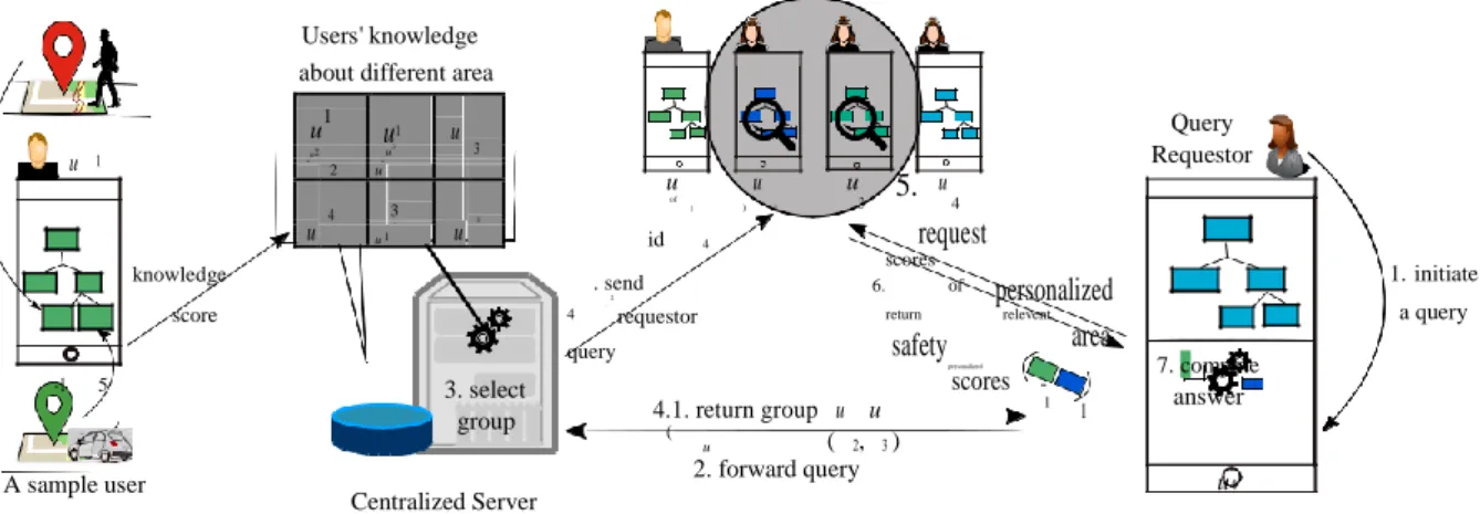
We develop a privacy-enhanced, personalized, and trustworthy solution for safe route planning with crowdsourced data and computation. Fig. 4.1 shows the architecture of our system. Users in our system store their pSSs of their visited areas on their own devices. In the case of storage constraints, users can also consider alternative private storage (cloud storage). The users share their KSs with the centralized server (CS). A KS only provides the information that a user has visited the area. A user can also hide the information of her visit on a sensitive area by not setting corresponding KS to 1 as the user has the control to decide on what the user shares with the CS.

In our system, we set a default ratio between the lengths of the safest and the shortest routes for the distance constraint. To initiate an SR query, the query requestor (QR) provides the source and the destination locations for the query. The QR can also specify the distance constraint as an absolute value or as a ratio between the lengths of the safest and the shortest routes. If the QR specifies the distance constraint, our system replaces the default distance constraint with the

15

(25)

4.2. QUANTIFICATION OF SAFETY 16

u ¹

knowledge

-1 5 score

A sample user

Users' knowledge about different area

u¹ u¹ ^u₃

u2 u³

u u

2 u

4 3 ₄

u u1 ⁴ u

3. select group

Centralized Server

u u

2

u

3

_5.u

4

of

1 )

id 4 request

scores

personalized

. send 6. of

2

requestor

.

4 return relevent

area

safety

query

personalized

(

,

)

scores - 4.1. return group u u ¹ 1

(

2 3

u

2. forward query

Query Requestor

7. compute answer

u4

1. initiate a query

Figure 4.1: System architecture

QR provided distance constraint. It is not realistic to use the computation power of all users for all queries and asking them whether they know any query-relevant area. The availability of KSs allows CS to address this issue. When the CS receives a query from a QR, it selects a group based on the query parameters and the stored KSs of the users. Then the CS returns the IDs of the group members to the QR and sends the identity of the QR to the group members. The QR evaluates the query in cooperation with the group members without involving the CS. The QR retrieves pSSs of the query- relevant area from the group members, computes the SSs of each road using the pSSs of the group members, and finds the SR. Note that the QR communicates with the group members in parallel to retrieve the pSSs. Therefore, the communication with multiple group members does not increase the query processing time significantly. However, in case of the resource constraint in the QR’s device, a subset of the group members’ pSSs can be retrieved.

4.2 Quantification of Safety

We utilize the personal travel experiences of the crowd to evaluate the SR queries. For this reason, we need to model the diverse travel experiences of each user into a personalized quantifiable metric of safety. In this section, we discuss our model for quantification of safety. We discuss the existing models that have quantified safety and their limitations in Section 4.2.1, and explain our safety quantification model in Section 4.2.2.

(26)

4.2.1 Limitations of Existing Models

Existing researches on safe routes have modeled safety in a variety of ways. The authors of [6, 7] quantify the safety of a road network edge by simply considering the number of crimes in the particular distance buffer area of that edge. They do not consider the recency and the severity of crimes, the ratio between the unsafe visits and the safe visits by an individual user, and the fact that the impact of a crime decays with distance. Thus, the quantified SSs of roads in [6, 7] fail to model the real-scenarios. The work in [4]

improves the way to find the SS of a road network edge by considering the crime events of the last few days and weighting the crime events based on their distances from the road. None of the above works [4, 6, 7] allow the SS to vary in different parts of a road network edge, which is possible for long roads.

In [8], the authors provide a more elaborate model of safety. However, the model suffers from the following limitations: (i) stores historical data and cannot address the constraint of the limited storage of the personal devices, (ii) does not differentiate the weights of crime events based on the frequency of the user’s visits, (iii) only considers that the effect of a crime spreads to its nearby places only if no crime occurs there, (iv) does not provide a smooth decay of the effect of older events, rather takes the moving average of the events of the last few days, and discards the impact of previous events, (v) does not consider the severity of a crime event, and (vi) does not allow the SS to vary in different parts of an edge.

4.2.2 Our Model

We develop a model that overcomes the limitations of existing models. In our model, the travel experiences of users are converted into pSSs and then aggregated to infer the SSs of different areas. When a user visits an area, an event occurs. If the user faces a crime, then that event is unsafe; otherwise, it is safe.

Model Properties

Our model has the following properties:

1. The safety of an area depends on the frequency of the users’ visits.

(27)

• If a user visits an area twice and faces unsafe events both times, then intuitively, that area is riskier than another area where a user visits 10 times and faces unsafe events two times among those visits.

• If a user visits an area 5 times safely, then that area is safer than another area that is visited once safely.

2. The safety of an area also depends on the safety of its nearby places. Therefore, if a user visits an area, the impact of the event is distributed to nearby areas.

3. The safety of an area depends on the recency of the safe and unsafe events. If a user faces an unsafe event in an area, then the crime’s effect decays with time. If a user visits an area safely, then the perception of safety due to the safe visit also decays with time.

4. The safety of an area depends on the type and severity of an unsafe event.

5. The pSSs are not allowed to grow indefinitely. They are bounded within a maximum and a minimum value so that while aggregating, a single user’s experience does not dominate the SS of an area.

6. A road network edge may go through multiple grid cells and thus, can have different SSs.

An important advantage of our model is that it is storage efficient as it does not store the historical visit data of a user.

Model Computation

Let the impact of a safe event in the occurring area be ₊ and the impact of an unsafe one be , where ₊; 2 N. ₊ is the same for all safe events. varies with the type and the intensity of the crime or inconvenience faced.

The impact (= ₊=) of an event reduces exponentially in nearby areas and becomes ⁰ as per the following equation: ⁰ = e ^dist_2h22

, where the constant h controls the spread of the event. dist represents the distance of the event location from the grid cell. This equation is inspired by the Gaussian kernel density estimation [4].

The pSS,of an area is bounded within [ S; S] and 2 N and 0 < + < S and S < < 0. If an event occurs in a place for the first time then = . If another event occurs there, then = + . If an event occurs nearby, whose effect is 0 here, then = + 0. If > S then = S and if < S then = S. Initially, is set to unknown.

(28)

4.3. INDEXING USER KNOWLEDGE 19

A pSS decays every

d days. If the decay rate is r_d and 6= 0, then after every

d days, becomes = r_d, where 0 < r_d < 1 and r_d 2 R. Therefore, the decay of older events’ impacts is smooth. For example, if r_d = 0:8 and _d = 2, then = 3 becomes 2.4 after two days, and becomes 1.92 after two more days.

The values of parameters ₊,, S+, S , _d and r_d are the same for all users and decided centrally.

For each grid cell, our model stores only two values: the pSS and when that pSS was last updated. Therefore, this model is storage-efficient and suitable for smart devices. The SS of an area is computed from the shared pSSs of the users (Definition 3).

4.3 Indexing User Knowledge

In this section, we elaborate on how we store the pSSs and KSs in our system. A user stores the pSS for every visited grid cell in the local storage and accesses it for evaluating the SR query. The CS stores the KSs of users for every grid cell and uses them for computing query-relevant groups.

For efficient retrieval of pSSs and KSs, we use indexing techniques: local and centralized, respectively. In Section 4.3.1, we explain the local indexing mechanism in detail, and in Section 4.3.2, we elaborate the global one.

4.3.1 Local Indexing.

Storing pSSs for the whole grid in a matrix would be storage-inefficient because a user normally knows about some parts of the grid area. We adopt a popular indexing technique R- tree [48] for storing pSSs of the visited grid cells. The underlying idea of an R-tree is to group nearby spatial objects into minimum bounding rectangles (MBRs) in a hierarchical manner until an MBR covers the total space.

For every visited grid cell, a user stores its pSS and the time of its last update. The last update time is required for decaying the pSS. To reduce the storage overhead, we combine nearby adjacent grid cells with an MBR, where the grid cells have the same SS and the difference between the last update times of two cells does not exceed a small threshold. We call this MBR as a supercell and each leaf node of an R-tree represents a supercell. Each leaf node stores the information of the coordinates of MBR, the pSS, and the average of the last update time of the considered grid cells of a supercell. The supercells are recursively combined into MBRs.

(29)

The intermediary nodes of the R-tree store the coordinates of the MBR. The MBR of the root node of the R-tree represents the total grid area. Fig. 4.2 shows an example of a grid and the corresponding R-tree. For the sake of clarity, we do not show the last update times in the figure.

Note that while creating supercells, there will be a small data loss due to the merging of grid cells for which the differences of their last update times are within a small threshold (e.g. in our experiment we set it to 12 hours).

yaxis

4 3 2

2 2

-1

3 -1

3 -2

-2

(0, 0)

(4, 4)

(0, 0)

(2, 0) (2, 4)

(4, 4) 1

3 3 3

0 1 2

3 4 x axis

(0,3) (2,4)

2 A

(1,0) (2,3)

3 B

(2,0) (4,1)

3 C

(2,1) (4,2) -2

D

(2,2) (3,4) -1

E

(a) The pSSs for a 4x4 grid is stored in a modified R-tree

yaxis

4 3 2

2 2 -1

3 -1

-2 -2 -2

(0, 0)

(4, 4)

(1, 0)

(0, 2) (4, 2)

(3, 4) 1

3 3 3

0 1 2

3 4 x axis

(1,0) (4,1)

3 C'

(1,1) (4,2)

-2

D'

(0,3) (2,4)

2 A

(2,2) (3,4) -1 E

(1,2) (2,3)

3 F

(b) A pSS changed from 3 to -2 and is updated in the R-tree Figure 4.2: A user’s pSSs is stored in a modified R-tree

(30)

Supercell Generation

A traditional R-tree only considers the location of the spatial objects for grouping, whereas we consider the location, the pSS and the last update time of the grid cells for grouping them into supercells. To compute the non-overlapping supercells, we scan the grid cells twice: row-wise and column-wise. For row-wise (or column-wise) scan, we maximize the number of grid cells included in a supercell row- wise (column-wise) and then take the supercells of the scan (row-wise or column-wise) that generates the minimum number of supercells. After computing the supercells for the leaf nodes, we insert them into a traditional R-tree.

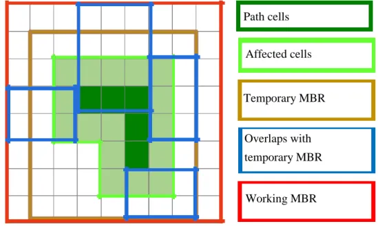
Supercell Update

Path cells

Affected cells

Temporary MBR

Overlaps with temporary MBR

Working MBR

Figure 4.3: Necessary MBRs for updating a supercell

To update the pSSs of grid cells for a visited route R, the following steps are performed:

• Compute route cells and affected cells. Compute the grid cells that overlap with R as route cells.

The affected cells include the route cells and their nearby cells (Fig. 4.3).

• Compute temporary MBR. Find the temporary MBR that includes the affected cells and one extra grid cell besides each affected cell in the boundary (Fig. 4.3). The reason behind considering an extra grid cell is to identify the adjacent existing supercells later.

• Find overlapping supercells. Find existing supercells that intersect with the temporary MBR. There are four overlapping supercells in Fig. 4.3.

(31)

4.4. QUERY EVALUATION 22

• Compute working MBR. Find the working MBR that includes these overlapping supercells and the affected cells (Fig. 4.3).

• Generate new supercells. By considering the location, the pSS and the last update time of the grid cells included in the working MBR, generate the new supercells.

• Update R-tree. Remove those overlapping supercells from R-tree and add the new supercells. Update the intermediary nodes based on the change in the leaf nodes. Fig.

4.2b shows the updated R-tree for the change of the pSS from 3 to -2 in a grid cell (shown with a red circle).

4.3.2 Centralized Indexing

The KSs are accessed when the query-relevant groups are computed and updated when a user visits a new area. Since the probability is high that at least a user knows a grid cell area, we store each grid cell’s data in a hash-map with the grid cell’s coordinates as a key. For each grid cell, we store the user ids whose KS is 1 for the corresponding grid cell area.

4.4 Query Evaluation

We elaborate our approach for finding the answer of an SR query in this section. We provide two optimal algorithms for computing an SR query. In Section 4.4.1, we calculate the query-relevant area and the query- relevant group for an SR query. This part is the same for both optimal algorithms. Then, in Sections 4.4.2 and 4.4.3, we describe two optimal algorithms, direct and iterative, respectively. After that, in Section 4.4.4, we analyze the complexity of our proposed algorithms. Next, in Section 4.4.5, we show the simulation of our algorithms for an SR query. Finally, in Section 4.5, we explain in detail the privacy-preserving aspects of our work.

In our system, a query requestor (QR) retrieves the required pSSs from relevant users and evaluates the SR query. We develop direct and iterative algorithms to find the SR for a source- destination pair s and d within a distance constraint .

The number of possible routes between a source-destination pair can be huge. Retrieving the pSSs for all grid cells that intersect the edges of all possible routes and then identifying the SR would be prohibitively expensive. Our algorithms refine the search space and avoid exploring all

(32)

routes for finding the SR. We present two optimal algorithms:

1. Direct Optimal Algorithm (Dir OA) 2. Iterative Optimal Algorithm (It OA)

Dir OA aims at reducing the processing time, whereas It OA increases privacy in terms of the number of retrieved pSSs. Though a pSS does not reveal a user’s travel experience (Chapter 4.5) with certainty, the user’s privacy is further enhanced by minimizing the number of shared pSSs with the QR.

4.4.1 Query-relevant Area and Group

Query-relevant area A_q.

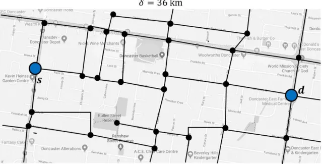
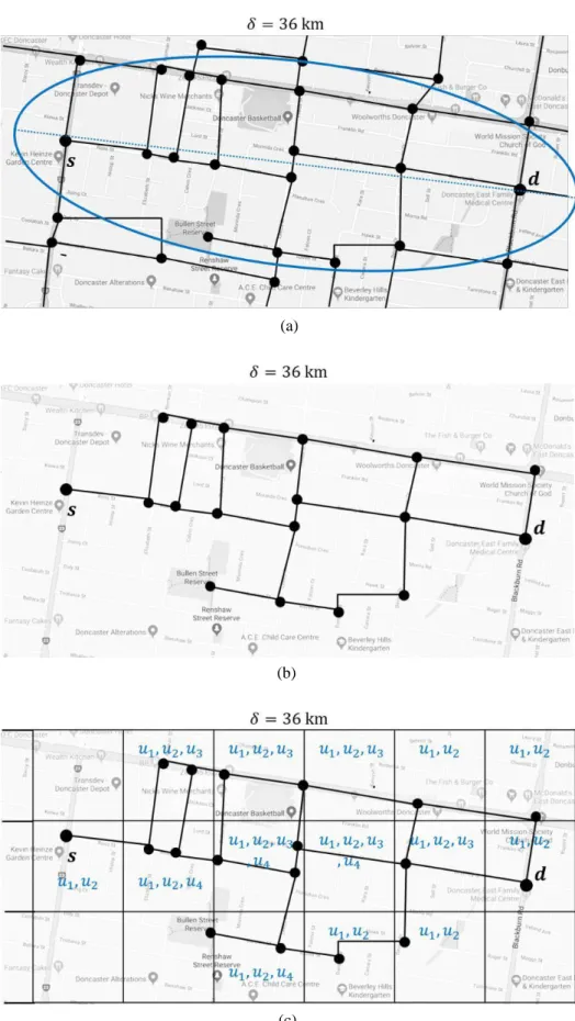
Our algorithms exploit the elliptical and Euclidean distance properties to find the query-relevant area A_q. We refine the search area using an ellipse where the foci are at s and d of a query and the length of the major axis equals . According to the elliptical property, the summation of the Euclidean distances of a location outside the ellipse from two foci is greater than the length of the major axis. On the other hand, the road network distance between two locations is greater than or equal to their Euclidean distance. Thus, the road network distance between two foci, i.e., s and d through a location outside the ellipse, is greater than . The refined search area A_q includes the grid cells that intersect with the ellipse. A_q enables us to select a query-relevant group and mitigate unnecessary processing and communication overheads and data exposure.

Query-relevant group G_q.

A query-relevant group G_q consists of the users whose KS is 1 for at least one grid cell in A_q. After receiving a query, the centralized server sends G_q and the list M_q of knowledgeable group members for every grid cell in A_q to the QR.

(33)

Algorithm 1: Dir OA(s, d, , N) compute query area(s; d; ; N);

retrieve query group(A_q);

compute SS(G_q; M_q; A_q);

4 N⁰⁰ refine query area(s; d; ; N⁰; SS_q);

5 SR compute safest route(s; d; ; N⁰⁰; SS_q);

6 return SR;

4.4.2 Direct Optimal Algorithm (Dir OA)

One may argue that we can simply apply an efficient shortest route algorithm (e.g., Dijkstra) for finding the SR by considering the SS instead of the distance as the optimizing criteria. However, it is not possible because the SR identified in this way in most of the cases may exceed .

Algorithm 1 shows the pseudocode for Dir OA. The algorithm starts by computing the query- relevant area A_q and the query-relevant road network N⁰ that is included in A_q. The edges in N that go through grid cells in A_q but those cells have not been visited by any user are not included in N⁰. Then the algorithm retrieves the query-relevant group G_q and the list M_q of grid cell wise knowledgeable group members from the centralized server. In the next step, the algorithm retrieves the pSSs from the group members and aggregates them to compute the SSs of the grid cell in A_q using Function compute SS.

After having the SSs for the grid cells in A_q, the algorithm further refines N⁰ to N ⁰⁰ by pruning the edges that are guaranteed to be not part of the SR (Line 4). The idea of this pruning comes from [4], where edges with the lowest SSs are incrementally removed until s and d become disconnected. To reduce the processing time, we exploit binary search for finding N⁰⁰. Specifically, we compute the mid-value mid of the lowest and the highest SSs, i.e., S and S, and remove all edges that have SS lower than or equal to mid. Note that an edge can have more than one associated SSs as it can go through multiple grid cells. For binary search, we consider the minimum of these SSs as the SS of the edge. After removing the edges, we find the shortest route between s and d and check if the length of the shortest route satisfies . If no such route exists, then the removed edges are again returned to N⁰⁰, and the process is repeated by setting the highest SS to mid. On the other hand, if such a route exists, the process is repeated by setting the lowest SS to mid + 1. The repetition of the process ends when the lowest SS exceeds the highest one.

Finally, Dir OA searches for the SR within in N⁰⁰ using Function compute safest route.

3 SS_q

2 G_q; M_q 1 N⁰; A_q

(34)

Dir OA starts the search from s and continuously expands the search through the edges in the road network graph N⁰⁰ until the SR is identified. The algorithm keeps track of all routes instead of the safest one from s to other vertices in N⁰⁰ as it may happen that expanding the SR from s exceeds before reaching d.

The compute safest route function uses a priority queue Q_p to perform the search. Each entry of Q_p includes a route starting from s, the road network distance of the route, the distance associated with each SS in the route. The entries in Q_p are ordered based on the safety rank, i.e., the top entry includes the SR among all entries in Q_p. Initially, routes are formed by considering each outgoing edge of s. Then the routes are enqueued to Q_p. Next, a route is dequeued from Q_p and expanded by adding the outgoing edges of the last vertex of the dequeued route. The formed routes are again enqueued to Q_p. The search continues until the last vertex of the dequeued route is d. While expanding the search we prune a route if it meets any of the following two conditions:

1. If the summation of the road network distance of the route and the Euclidean distance between the last vertex of the route and d exceeds .

2. If the road network distance of the route exceeds the current shortest route distance of the last vertex from s.

Both pruning criteria guarantee that the pruned route is not required to expand for finding the SR. The current shortest route in the second pruning condition for a vertex v from s is determined based on the distances of the dequeued routes whose last vertex is v. Since the dequeued routes to v are safer than a route that has not been enqueued yet, the route can be safely pruned if its length is greater than the current shortest route’s distance.

4.4.3 Iterative Optimal Algorithm (It OA)

It OA enhances user privacy by reducing the shared pSSs with the QR as it does not need to know the SSs of all grid cells in A_q. Algorithm 2 shows the pseudocode for It OA. Similar to Dir OA, It OA computes N⁰, A_q, G_q, and M_q. It OA does not apply the binary search to further refine N⁰ as it avoids retrieving the pSSs of all grid cells in A_q. It OA gradually retrieves the pSSs from the group members only for the grid cells that are required for finding SR. Another advantage of It OA is that it only involves those group members who know about the required grid cells.

(35)

Algorithm 2: It OA(s, d, , N)

1

N⁰; A_q compute query

area(s; d; ; N);

2 G_q; M_q retrieve query group(A_q);

3 SSq ;, Q_p ;, v s;

4 while v! = d do

5 A_q⁰ find required cells(v; N⁰; A_q; SS_q);

6 SS_q SS_q

S

compute SS(G_q; M_q; A_q⁰);

7 SR get safest route(v; N⁰; SS_q; Q_p);

8 v get last vertex(SR);

9 return SR;

It OA iteratively searches for the SR in N⁰ using a priority queue Q_p like Dir OA. It OA expands the search by exploring the outgoing edges of v. Initially v is s and later v represents the last vertex of the dequeued route from Q_p. In each iteration, It OA identifies the grid cells in A_q⁰ through which those outgoing edges pass (Function find required cells), and computes their SSs by retrieving pSSs from the group members (Function compute SS). Next, using Function

get safest route, It OA forms the new routes by adding the outgoing edges of v at the end of the last dequeued route, and enqueues them into Q_p if they are not pruned using the conditions stated for Dir OA. At the end, the function dequeues a route from Q_p for using that in the next iteration. The search for SR ends if the last vertex of the dequeued route is d.

It OA increases the communication frequency of the QR with the relevant group members. To mitigate this issue, we introduce a parameter X_it that trades off between the communication frequency and the number of pSSs shared with the QR. For X_it = 1, the algorithm considers only the outgoing edges of the last vertex v of the dequeued route for identifying the grid cells for which the pSSs will be retrieved. For X_it > 1, the algorithm repeats the process X_it times by considering the outgoing edges of the last vertices of the newly formed routes. While doing

so, the algorithm applies the first and second pruning techniques where applicable. We decide the value of X_it in experiments. Please note that the algorithm do not collect the pSSs of nearby edges if the SSs of the immediate edges to be expanded are known.

4.4.4 Complexity Analysis

The compute safest route function in Dir OA algorithm can be drawn as a tree where the source node is the root and the destination node is in the last level. If the average branching factor is b

A PRIVACY-ENHANCED APPROACH FOR PLANNING SAFE ROUTES WITH CROWDSOURCED DATA AND

M.Sc. Engg. (CSE) Thesis