MULUGETA AKLILU ZEWDIE
GRADUATE SCHOOL
BOGOR AGRICULTURAL UNIVERSITY
BOGOR
I declare that this thesis is my original work and that all resources of materials used for this thesis have been duly acknowledged. This thesis has been submitted to Graduate School Department of Statistics Bogor Agricultural University in partial fulfillments of the requirements for M.Sc. degree in Statistics. I seriously declare that this thesis has not been submitted to any other institution and anywhere for the award of any academic, degree, diploma, or certificate.
Bogor, Oct. 2015
iv
SUMMARY
MULUGETA AKLILU ZEWDIE.Spatial Econometrics Model of Poverty in Java Island. Advised by. MUHAMMAD NUR AIDI and BAGUS SARTONO.
Poverty means people's basic needs like food, clothing, and shelter are not being met. It is generally of two types: Absolute poverty and Relative Poverty: absolute poverty is synonymous with destitution and occurs when people cannot obtain adequate resources (measured in terms of calories or nutrition) to support a minimum level of physical health. Relative poverty occurs when people do not enjoy a certain minimum level of living standards as determined by a government (and enjoyed by the bulk of the population).
In poverty model Spatial analyses treated the violation of assumption of independence of error term and play a very important role because if we use multiple linear regression model that exclude explicit specification of spatial effects, when it is exist, can lead to inaccurate inferences about predictor variables. Moran Index test is applied to test for the existence of spatial autocorrelation among district poverty rates and confirm the existence of spatial effect. The Weighted matrix is obtained by using queen contiguity criteria. Model selection is also one of predominant issue in spatial econometric model. The Likelihood Ratio common factor test, Robust LM test and AIC are used for model selection criteria. The SAR model proved to be better than the other model for a given data.
Finally this paper gives you the concept of spatial econometric model on poverty and applies it to analyze the spatial dimensions of poverty and its determinants using data from Java Island 2010 census survey, for 105 districts of Java Island. Dependent variable used in this research is percentage of poverty rate at particular district and predictors are some selected variables those are correlated to poverty. Weighted matrix is obtained by using queen contiguity criteria and four statistical models are applied to the data, multiple linear regression models, Spatial Error Model, Spatial Lag Model and Spatial Durbin Model. It is shown
MULUGETA AKLILU ZEWDIE.Spasial Ekonometrika Model Kemiskinan di Pulau Jawa. Dibimbing oleh. MUHAMMAD NUR AIDI dan BAGUS SARTONO.
Kemiskinan merupakan kebutuhan dasar masyarakat seperti makanan, pakaian, dan tempat tinggal yang tidak terpenuhi. Hal ini umumnya dibagi menjadi dua jenis: kemiskinan mutlak dan kemiskinan relatif: kemiskinan mutlak dapat diartikan dengan keadaan orang yang tidak memperoleh sumber daya yang memadai (diukur dari segi kalori atau nutrisi) untuk mendukung tingkat minimum kesehatan fisik. Kemiskinan relatif terjadi ketika orang tidak menikmati tingkat minimum standar hidup tertentu yang ditentukan oleh pemerintah (dan dinikmati oleh sebagian besar penduduk).
Dalam analisis model spasial, kemiskinan harus memenuhi pelanggaran asumsi independensi jangka kesalahan. Jika menggunakan model regresi linier berganda yang didalamnya tidak terdapat efek spasial yang spesifik, maka dapat menyebabkan ketidak akuratan inperensis pada variable predictor. Moran indeks test digunakan untuk menguji keberadaan autokorelasi spasial pada data kemiskinan ditingkat kabupaten dan hasilnya terdapat autokorelasi pada data kemiskinan tersebut. Pembobotan matrik menggunakan kriteria pendekatan Queen. Pemilihan model, didalam analisis ini menggunakan uji factor Likelihood Ratio, Robust LM (Lagrange multiplier) dan AIC (Akaike’s Information criteria). Penelitian ini memberikan konsep model ekonometrika spasial kemiskinan dan berlaku untuk menganalisis dimensi spasial kemiskinan. Data yang digunakan merupakan hasil survey pada tahun 2010 dari 105 kabupaten di Pulau Jawa. Variabel dependen yang digunakan dalam penelitian ini adalah persentase tingkat kemiskinan di tingkat kabupaten dan variable independen merupakan beberapa variable yang berhubungan dengan kemiskinan. Dari pembobotan matrik yang menggunakkan pendekatan Queen dan empat model statistic yang digunakan pada data, analisis model regresi berganda, analisis model eror spasial, analisis model spasial Lag dan analisis model spasial Durbin, menunjukkan bahwa estimasi OLS (ordinary least square) pada model kemiskinan belum memenuhi salah satu asumsi regresi. Oleh karena itu dibutuhkan analisis spasial ekonometrika model. Setelah penggunaan spasial ekonometrika model, asumsi Gauss Markov telah terpenuhi dan hal ini menunjukkan analisis spasial Lag model lebih baik daripada analisis model lainnya untuk data kemiskinan. Hasil dari penelitian ini menunjukkan bahwa tingkat pendidikan dan jam kerja memiliki dampak yang signifikan terhadap kemiskinan.
vi
Copyright © IPB 2015
Copyright © IPB 2015
viii
SPATIAL ECONOMETRICS MODEL OF POVERTY IN JAVA
ISLAND
MULUGETA AKLILU ZEWDIE
Thesis
In the partial fulfillment of the requirements of the degree of Masters of Science
in Statistics
GRADUATE SCHOOL
BOGOR AGRICULTURAL UNIVERSITY
BOGOR
ACKNOWLEDGMENTS
Thanks and Praise to the Living triune God who guided, provided and sustained me with wisdom, courage and perseverance throughout this journey.
Next I would like to deeply thank my advisors Dr. Ir. Muhammad Nur Aidi and Dr. Bagus Sartono for their valuable advice and constructive comments in while working this thesis, and throughout accomplishment of my entire career in IPB.
From my heart, I would like to express my gratitude to the government of Indonesia for financial support during my study in IPB and specially department of statistics for providing me the opportunity of doing my M.Sc. study.
Finally my deep thanks go to all my family, colleagues and others who encouraged me in various aspects while conducting this Thesis.
ii
TABLE OF CONTENTS
TABLE OF CONTENTS i
LIST OF ABBREVIATIONS iii
LIST OF TABLES iv LIST OF FIGURES iv LIST OF APPENDICES iv 1.INTRODUCTION 1
Background 1
Statement of the Problem 3 Objective of the Study 3 Significance of the Study 3 2.LITERATURE REVIEW 4 Multiple linear regression 5 Weighted Matrix 5
Test Spatial Autocorrelation 6
Spatial Econometric Models 6 Spatial Lag Model 7
Spatial Error Model 7
Spatial Durbin Model 7
Test for Assumptions 10
Model Selection 11
3.RESEARCH METHODS 11
Description of Study Area 11
Data 11
Dependent Variable 12
Independent Variables 12
Steps of Analysis 12
4.RESULTS AND DISCUSSION 14
Descriptive Statistics 14
Global vs Spatial Econometric Model 16
5.CONCLUSIONS AND RECOMMENDATIONS 18
Conclusions 18
Recommendations 18
REFERENCES 19
APPENDICES 20
LIST OF ABBREVIATIONS
AIC Akaike’s Information criteria
SAR Spatial Autoregressive
SEM Spatial Error Model
SDM Spatial Durbin Model
SAC Spatial Autocorrelation Model
DW Durbin Watson
LM Lagrange Multiplier RLM Robust Lagrange Multiplier
OLS Ordinary Least Squares
iid Independent and identically distributed RI Republic of Indonesia
iv
LIST OF TABLES
Table 1: MoranTest, LM vs RLM tests 15 Table 2: Spatial Vs Global Model 16
Table 3: Assumption Tests 17
LIST OF FIGURES
Figure 1: Conceptual Figure of the Entire Model 8 Figure 2:Methods of Analysis in Flow Chart 13
Figure 3: Percentage of Poverty Rate in Java Island 14
LIST OF APPENDICES
Background
Poverty is pronounced deprivation in well-being meaning people's basic needs like food, clothing, and shelter are not being met. Poverty is generally of two types: (1) Absolute poverty is synonymous with destitution and occurs when people cannot obtain adequate resources (measured in terms of calories or nutrition) to support a minimum level of physical health. Absolute poverty means about the same everywhere, and can be eradicated as demonstrated by some countries. (2) Relative poverty occurs when people do not enjoy a certain minimum level of living standards as determined by a government (and enjoyed by the bulk of the population) that vary from country to country, sometimes within the same country. Relative poverty occurs everywhere, is said to be increasing, and may never be eradicated. The measurement and analysis of
poverty and inequality is crucial for understanding peoples’ situations of well -being and factors determining their poverty situations. A poverty profile describes the pattern of poverty, but is not principally concerned with explaining the causes of poverty. Yet, a satisfactory explanation of why some people are poor is essential if we are to be able to tackle the roots of poverty. Among the key correlates, of poverty are region-level characteristics, which include vulnerability to flooding or typhoons, Remoteness, quality of governance, and property rights and their enforcement. Community-level characteristics, which include the availability of infrastructure (roads, water, electricity) and services (health, education), proximity to markets, and social relationships. Household and individual characteristics, among the most important of which are
a. Demographic, such as household size, age structure, dependency ratio, gender of head.
b. Economic, such as employment status, hours worked, property owned. c. Social, such as health and nutritional status, education, shelter.
2
Halving the number of people living in less than a dollar a day by 2015 was the key focus of the Millennium Development Goals agreed to at the Fifty-fifth session of the General Assembly of the United Nations and subsequently adopted by leading development institutions. They have inspired unprecedented efforts to meet the needs of the worlds poorest and have focused attention on the issue of poverty reduction amongst the most poor. Yet, despite the progress that has been, made recent estimates suggest that between 300 million and 420 million people in the world are living in chronic poverty (McKay & Lawson 2003)while currently this number is increased.
Poverty is one of the fundamental problems that become the center of attention of the governments of all countries in the world, especially for developing countries like Indonesia. As National Development Planning Agency (Bappenas 2010) report peoples living below poverty line in Indonesia is still quite large. In 2010, Bappenasas figured the numbers of poor people in Indonesia are around 31.02 million. Additionally, Bappenas noted that as much as half of the total percent or around 55.83% of the total poor population in Indonesia settled in Java Island (Bappenas 2010).Java Island is the most populous island in Indonesia. It consists of 6 provinces namely the Special Capital Region of Jakarta, West Java, Banten, Central Java, Yogyakarta and East Java. Each province consists of several districts. One of the efforts made to address the problem of poverty is to identify the variables that affect poverty on these districts. The poverty of the district due to the impact of poverty in the surrounding district indicates a spatial
effect. Based on the first law of Geography, “everything is interconnected to each other, but something close more influence than something far”. (Lee et al.2001).
Indonesia's poverty line is determined by a complex function taking in what the poor spend on different kinds of food to reach 2.100 calories per day, as well as costs associated with dozens of non-food goods, including housing, clothing, education and health care. The poverty line is established as an average, allowing for the fact that prices vary widely from urban to rural areas, and from more prosperous Indonesian regions. Based on the government's official poverty line is 233.740 rupiah per capita per month which is close to UN poverty line measurement from 1-2 dollar a day.
A spatial analysis framework offers advantages over tabular analysis. From spatial analysis perspective Poverty maps are important tools that provide information on the spatial distribution of poverty. It used to affect various kinds of
decisions, ranging from poverty alleviation programmers’ to emergency response
and food aid. The Visualization of the estimates in map form is an efficient medium for planning responses to poverty. Spatial statistics can quantify and clarify patterns seen in maps. A spatial framework allows for incorporating spatially continuous environmental variables in the analysis. Explicit spatial analyses take into account the local nature of relationships between poverty and its determinants. However, the use of poverty maps alone does not furnish an estimate of the causal linkage between poverty and the variables influencing it;
such maps furnish only “visual” advice. For this reason, researchers usually look
regression models for cross-sectional and panel data. It is the result of the development of the classical linear regression method. The development was based on the presence or influence of a spatial effect.
Statement of the Problem
Most of the researcher in the analysis of poverty they used classical linear regression model however the result gives less precise because of the nature of poverty data contains spatial effect so that the model will be less accurate and led to the conclusion that less precise due to the assumption of independent errors and homogeneity assumptions are not met. Therefore, the need for a more accurate analysis on spatial data is spatial econometric model. In this research, modeling and analysis of the poverty data which has spatial effect can be used spatial Econometric model.
Objectives
Main objective
The main objective of this research is to identify the variables that affect poverty by applying Spatial Econometric Model in Java Island with105 districts.
Specific Objective
a. To identify the variable that significantly determine poverty b. To make policy recommendation to prevent and alleviate poverty
c. To compare the best model among classical linear regression and Spatial Econometric Models
Significance of the Study
a. The outcomes of the analysis are used to inform policy making as well as in designing appropriate model and for assessing effectiveness of on-going policies and strategies on the reduction of poverty.
b. Can be used as source of methodological approach for studies dealing on the spatial econometric model.
4
2.
LITERATURE REVIEW
Nelson Mandela came out of retirement in February 2003 to speak on behalf of to Make Poverty History campaign in London, an effort to renew the global
commitment to eliminating poverty worldwide. “Like slavery and apartheid,
poverty is not natural”, Mandela intoned. “It is man-made, and it can be overcome
and eradicated by the action of human beings.” In imagining a world without poverty, hope that Mandela’s strong voice will spur surer action to eliminate the deprivations suffered by the world’s poor.
Statistical offices spend much time and effort setting and updating poverty lines. However, the place of poverty lines needs to be put in context. A recent study of 17 Latin American countries, for example, shows that many other elements of poverty measurement are more important than the choice of poverty lines. These include adjustments for adult equivalent family size and the treatment of missing data in surveys is important rather than choosing poverty line. (Szekely
et al. 2000).
Over the past many years, the causes and consequences of poverty, and changes in poverty over time, have been the subjects of much academic research and social policy debate. In large measure, two schools of thought have dominated this research and debate. One attributes the causes of poverty primarily to
individualistic or family compositional forces. Sometimes referred to as “people poverty”, another school of thought focuses on contextual or structural forces, sometimes referred to as “place poverty.” These include issues such as urban economic dislocations, faltering regional economies, high unemployment, poor and often disorganized local employment opportunity structures all forces over which the individual has little or no control. (Pebley & Sastry 2003).
A key element affecting poverty is regionalism; Said Levernierand concluded that economic development targeting predominantly African-American
Multiple Linear Regressions
Simple linear regression model is not adequate for modeling many economic phenomena, because in order to explain an economic variable it is necessary to take into account more than one relevant factor. Multiple linear regressions is given by the following expression: (Rawling et al. 1998)
: Random error term iid with mean zero and constant variance.
When conducting regression analyses with data aggregated to geographic areas such as an irregular lattice, it is common to find spatially auto-correlated residuals. When spatial autocorrelation exists, in multiple linear regressions above; the error term has to take the autocorrelation into account. (Anselin 2001) and look for spatial models would be prefer because Ordinary Least Squares (OLS) in multiple linear regression analysis, the resulting parameter estimates are biased, inconsistent and the R square values is not an accurate fitness of fit measure due to violation of assumption that was explain in the problem of statement.
Weighted Matrix
The basis for most models is an indicator of whether one region is a spatial neighbor of another; or equivalently, which regions are neighbors of a given region. This is a square symmetric weighted matrix (W) nxn (row standardized) matrix that define who are neighbours with who. To construct this weighted matrix:
1) Contiguity based weighted matrix: Queen 2) Inverse Distance weighted matrix
3) K –nearest neighbor weighted matrix
6
Spatial autocorrelation stems from "similarities" between neighboring clusters; there is autocorrelation when the covariance between "neighboring" cluster i and cluster j does not equal zero, and no autocorrelation exists otherwise .One of the most common tests for the existence of spatial autocorrelation (measures is Global Moran's I which depends on a "weight matrix" at particular data residual or vector
y.Moran test statistics for spatial autocorrelation is as follows:
)
When significant spatial autocorrelation, (spatial dependence) exists either globally or locally, spatial heterogeneity exists and accordingly non constant errors.(Anselin 1988; Higazi et al. 2013)
Spatial Econometric Models
Spatial data is characterized by having "location" or "Spatial" effects, where there is spatial heterogeneity between and spatial homogeneity within
neighboring clusters; thus “spatial dependence" is exhibited among these clusters.
Spatial Autocorrelation Model
The spatial autocorrelation model is a combination of spatial lag effect model and spatial error models which calls most of time Simultaneous autoregressive model or general spatial model according to (Lesage 2009) and (Paraguas & Kamil 2005) is as follows:
.
With: ; ε~N(0,2I) Where: =the spatial error coefficient; =spatial lag coefficient
W=n Xn spatial weight matrices
From the Spatial Autocorrelation model restricting the spatial error effects
parameters equal to 0 can derive other models SAR. Meaning λ= 0, a “spatial lag”
model or following SAR model can be derived which is analogous to the time-series lagged dependent variable is:
ε~N(0,2I) Spatial Error Model (SEM)
When ρ in Spatial Autocorrelation model is set to 0, a spatial error model (SEM) with spatial effect of error term can be derived the form:
ε~N(0,2I)
Since in the likelihood ratio common factor test according to Elhorst’s flow chart if the null hypothesis accepted lamda will be equal to rho so the model can be write in above form.
Spatial Durbin Model (SDM)
Spatial Durbin Model according to (Lesage 1999) is:
8
Xj Xi Xj Xi Xj Xi Xj Xi
Ɛj Ɛi Ɛj Ɛi Ɛj Ɛi
Ɛj Ɛi No influence from neighbors
Dependent variable Influenced by
neighbors
Residuals influenced by
neighbors
Independent variable influenced by
neighbors Under SDM by using likelihood ratio common factor we can come out to SEM model & SAR model.H0: if it is not significant our model goes to SEM.if it is significat it will be SAR or OLS depending on spatial lag coeeficients here is the concept:
The entire above all models uses Maximum likelihood estimation for the parameters beta and teta.
Conceptual figure of the above all model are as follows:
Figure 1. Conceptual Figure of the Entire above Model
Yj Yi
Yj Yi Yj Yi Yj Yi
There are several diagnostic tests that could be used to test the Significance of spatial effects; these are Lagrange Multipliers (LM lag test and LM-error) to tests spatial dependences. Also residual plots and residual maps are also examined to locate extreme values and reveal heterogeneity, globally and locally. According to Anselin (2010) the Lagrange Multiplier Test for Spatial Error (LM-ERR) hypothesis is as follows: H0 :
= 0 (no spatial error effect )H1:
≠ 0( there is spatial error effect) The Lagrange Multiplier test statistics for this is:
The next Lagrange Multiplier Test for Spatial Lag (LM-Lag) hypothesis is : H0:
= 0 (there is no spatial lag effect)H1:
≠ 0 ( there is spatial lag effect ) The Lagrange Multiplier test statistics for this is:] and log-likelihood function of the restricted model respectively. (Mur & Angulo 2006) Reject/accept by using p-value criteria.
Test for Assumptions of Error Term
10
a. Homogeneity of error Term
V (εj ) = σ2 for all j. That is, the variance of the error term is constant. (Homoskedasticity). If the error terms do not have constant variance, they are said
to be heteroskedastic. [Tidbit from Wikipedia: The term means “differing variance” and comes from the Greek “hetero” ('different') and “skedasis”
('dispersion').]Breusch pagan test is one of the test statistics to test it and Hypothesis are as follows: H0: Homoscedasticity H1: hetroscedasticity
With Test statistics where SSR(explained sum squared /sum squared distribution H1: residual is not normal distribution .(Arbia, 2006) as stated the test statistics is:
Where Fn(x) = being the empirical cumulative distribution function based on
n observations
F0(x) = the theoretical cumulative distribution function under the null hypothesis Reject H0 if |k| > q (1- α)
c. Independent of error term
Model selection can be helpful to identify a single best model or to make inferences from a set of multiple competing hypotheses Up to now, however, only a few model selection procedures have been tested for spatially auto correlated and spatial lag data. Therefore the researcher developed model selection procedures and selected the best models among OLS, SDM, SAR and SEM by model selection criteria of akaike information criteria (AIC) as follows:
Where p is the number of coefficients in the regression equation, normally equal to the number of independent variables plus 1 for the intercept term.
3. RESEARCH METHODS
Description of Study Area
Indonesia is a large Southeast Asian country with 497 regencies and administrative cities spread out in 33 provinces. The country is an archipelago consisted by big five island (Java, Sumatera, Kalimantan, Sulawesi and Papua) beside more than 17 thousand small islands hemmed in the Atlantic Ocean in the Northern edge and the Indian Ocean in the Southern edge. The researcher interest goes to the most populated Island named Java Island which has 6 provinces namely the Special Capital Region of Jakarta, West Java, Banten, Central Java, Yogyakarta and East Java. Each province consists of several districts. However the researcher only takes under consideration of 105 districts.
Data
The data is secondary data which is collected by BPS Indonesia, in 2010. All the response and explanatory variables are continuous and all variable are changed to percentage for analysis purpose.
Dependent Variable
12
Independent Variables
The explanatory variables that are included in this study by assumed to be correlates to poverty are:
X1: Percentage Unemployment rate X2: Percentage Malnutrition rate X3: Percentage Child mortality rate
X4: Percentage Morbidity (occurrence of disease) X5: Percentages of household more than high school X6: Percentage of access to clean water
X7: Percentage of non-sanitation X8: Percentage Literate rate X9: Percentage Employment rate
X10: Percentage of un worked hour per week X11: Percentage health complain of the household X12: Length of sickness
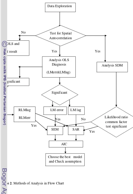
Methods of Analysis
1. Data exploration with graph and descriptive statistics: this part explain descriptive part of the analysis by using bar chart of the given province data without considering the districts so that can know the general outline of poverty in java island.
2. Analysis Multiple linear Regression model using OLS estimation: In this part all we want to compare the global model by using ols estimation after that we want to extract the error to check the assumption.
3. Create row standardized weighted matrix Using contiguity Queen Criteria: the row standardized matrix helpful before go to the spatial part must be created here by looking Queen Criteria refer more detail for this matrix in the Research reviews.
4. Test for the existence of spatial autocorrelation using Moran Index test :
After we get the weighted matrix we want to know about the spatial correlation since spatial correlation can affect the result of multiple linear regressions so that Moran I test will be held on here.
5. Test for spatial lag and spatial error effect by using LM and Robust LM test If the spatial effect occurs we need to identify the source of its effect by using Lagrange multiplier Test.
6. Analysis Spatial Lag Model, Spatial Error Model and SDM model
The analysis our Spatial Econometrics model so far we already identified the effects of spatial models in the existence of autocorrelation
7. Under spatial Durbin model test LRcom factor test and come up to the reduced model: likelihood ratio common factor test is very important to identify our best model.
No
Yes Yes
Yes No Yes
Yes
Figure 2. Methods of Analysis in Flow Chart All significant
Choose the best model and Check assumption
Analysis SDM Data Exploration
Analysis OLS Diagnosis (LMerr&LMlag) Analysis M-OLS and
Keep M-OLS result
LM lag LM error
AIC Test for Spatial Autocorrelation
Significant
Likelihood ratio common factor
test significant Robust LM
Significant
RLMlag RLMerr
14
4.
RESULT AND DISCUSSIONS
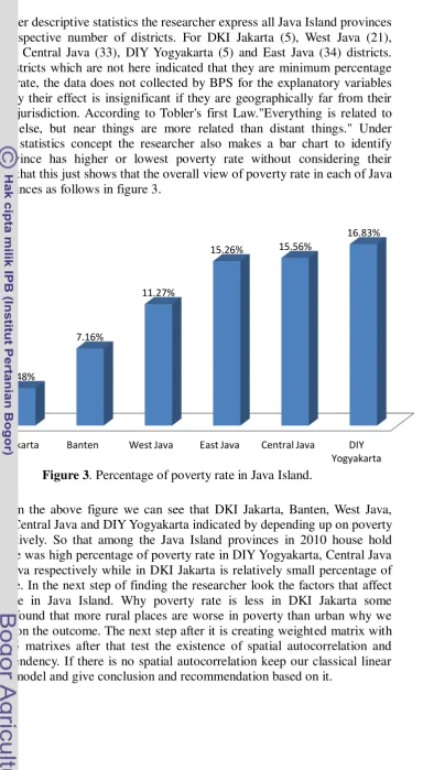
Under descriptive statistics the researcher express all Java Island provinces with the respective number of districts. For DKI Jakarta (5), West Java (21), Banten (7), Central Java (33), DIY Yogyakarta (5) and East Java (34) districts. The rest districts which are not here indicated that they are minimum percentage of poverty rate, the data does not collected by BPS for the explanatory variables and spatially their effect is insignificant if they are geographically far from their
neighbor’s jurisdiction. According to Tobler's first Law."Everything is related to everything else, but near things are more related than distant things." Under descriptive statistics concept the researcher also makes a bar chart to identify which province has higher or lowest poverty rate without considering their districts so that this just shows that the overall view of poverty rate in each of Java Island provinces as follows in figure 3.
From the above figure we can see that DKI Jakarta, Banten, West Java, East Java, Central Java and DIY Yogyakarta indicated by depending up on poverty rate respectively. So that among the Java Island provinces in 2010 house hold survey there was high percentage of poverty rate in DIY Yogyakarta, Central Java and East Java respectively while in DKI Jakarta is relatively small percentage of poverty rate. In the next step of finding the researcher look the factors that affect poverty rate in Java Island. Why poverty rate is less in DKI Jakarta some researcher found that more rural places are worse in poverty than urban why we shall get it on the outcome. The next step after it is creating weighted matrix with 105 by 105 matrixes after that test the existence of spatial autocorrelation and spatial dependency. If there is no spatial autocorrelation keep our classical linear regression model and give conclusion and recommendation based on it.
DKI Jakarta Banten West Java East Java Central Java DIY
Yogyakarta 3.48%
7.16%
11.27%
15.26% 15.56%
16.83%
Moran Index Test for autocorrelation
Moran I statistic standard deviate = 8.464, p-value < 2.2e-16 Moran I statistic Expectation Variance
0.5596 -0.0096 0.0045
Lagrange multiplier diagnostics for spatial dependence LMerr = 19.016, df = 1, p-value = 1.296e-05
LMlag = 27.620, df = 1, p-value = 1.477e-07
Robust Lagrange multiplier diagnostics for spatial dependence RLMerr = 0.0015, df = 1,p-value = 0.9691
RLMlag = 8.6051, df = 1, p-value = 0.0034
From the above table 1 Moran I test statistics (0.56) indicated that there is a positive autocorrelation in this poverty data. And the researcher test the significant of autocorrelation by looking p value (2.2e-16) that is very small and less than 0.05 so reject the null hypothesis as stated in the research methods and we conclude that there is a positive spatial autocorrelation in the given poverty data meaning high values of a poverty rate at one locality are associated with high values at neighboring localities or low values of a poverty rate at one locality are associated with low values at neighboring localities since the spatial
autocorrelation is positive. In another way Moran’s I (0.56) can be interpreted as
16
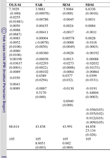
is spatial lag model. So from it as we can see that literate rate and house hold who has higher education is a negative impact on poverty while employer who has more un worked hours per week has a positive impact on poverty. In our lag model the spatial lag effect is significant (0.51702) which mean that on average 100 percent increased in poverty rate in a location resulted in 51.7 percentage point increase in poverty rate in neighbors location and the highest significant of error lag also indicated that a random shocked in spatially omitted variable that affects percentage of poverty rate in a particular location triggers a change in percentage of poverty rate. The next thing is to check our best model to fulfills the requirement of assumptions remember the dependent variable was change to log since the residuals have a skewed distribution. The purpose of a transformation is to obtain residuals that are approximately symmetrically distributed (about zero, of course),all the non bracket page with respect to each model shows the value of the variable is insignificant and under bracket of above table shows p value. Table 3.Assumptions Test SAR/lag model enough to say that our model has no problem on normality assumption, From KS test we can also conclude that our model is normal distributed since (KS=0.095238 with p-value=0.7277) indicated that we accept the null hypothesis so that there is no normality problem in our model. For more the researcher also tested the constant variance assumption here the result above from BP test indicated that there is no more heterogeneity problem since the p value is greater than 0.05 we accept the null hypothesis that mean the variance is homogen. Remember as stated before in the research methods our null hypothesis is homoscedasticity against hetroscedastcity.The OLS result of Durbin Watson is 1.56 which indicates that residual are auto correlated so that the OLS model will not accurate since this assumption violated while the SAR model as we seen above table DW=2.24 is greater than du that means there is no problem of
18
5.
CONCLUSION AND RECOMMENDATION
Conclusion
Global Econometric model has largely ignored spatial dependency between the observations and spatial heterogeneity in the relationship we are modeling, because they violate the Gauss-Markov assumptions used in regression modeling. A major assumption that is never satisfied when variables are from contiguous observations is the independence of error terms. Spatial analyses treated the violation of this assumption and play a very important role because global Models that exclude explicit specification of spatial effects, when it is exist, can lead to inaccurate inferences about predictor variables. Based on it between Global and Spatial Econometric model the researcher found that the best model is spatial model in the existence of spatial autocorrelation obviously in case of spatial dependence and heterogeneity to full fill all the required assumptions. Among all models the best one for this poverty data is Spatial lag model.
As we know poverty is a complex phenomenon we cannot determine it
within a short period of time if we don’t know the significant determinant factors
but if we know the significant factors to reduce poverty so that we can easily fight it. In this research the researcher found that based on the best model (spatial lag model) the literate rate, house hold who have higher degree and employer unworked hours are significant determinate factor of poverty as we see on the output of spatial lag model. The parameter of literate rate is negative which indicated that poverty and literate rate has a negative relationship that mean the more we are educated we can alleviated poverty as well, the more we are illiterate the more we are poor while employer un worked hours are a positive relationship that indicated the more we have un worked hours or spent our working time without doing our activity the more we are poor.
Recommendation
As individual level the researcher recommend to the household of all family member must be increase there working time if they are whatever government employer or private employer so that it can help to generate income and alleviate poverty.
As a government level the researcher recommended that the policy must focused on developing human capacity by increasing literacy rate and education should be free and supported by government until strata one so that educated people can be alleviate poverty in many direction.
Anselin L.1988. Spatial Econometrics: Methods and Model, Kluwer, Dordrecht. Anselin L.2001.Spatial Econometrics in a companion to Theoretical Econometrics
( Baltagi B.H. ed). Blackwell.Oxford.
Anselin L.2010.Lagrange multiplier diagnostics for spatial dependence and heterogeneity, Geographical Analysis. Wiley online library.
Arbia G. 2006.Spatial Econometrics Statistical Foundations and Applications to Regional Convergence, Italy.
[BAPPENAS] National Development Planning Agency. 2010. Report on the Achievement of the Millennium Development Goals Indonesia.
Coudouel A, Jesko H, Quentin W. 2002. Poverty Measurement and Analysis, in the PRSP Sourcebook, World Bank, Washington D.C.
Harrison A. 2007.Globalization and Poverty, NBER Books, National Bureau of Economic Research.
Hentschel J, Lanjouw P, Poggi J. 2000. Combining census and survey data to trace the spatial dimensions of poverty: a case study of Ecuador. World Bank Econ.
Higazi SF, Abdel-Hady DH, Al-Qulfi SA. 2013. Application of Spatial Regression Models to Income Poverty Ratios in Middle Delta Contiguous Counties in Egypt.Tanta University, Tanta, Egypt
Lee J, David W. 2001. Statistical analysis with arc view GIS, John Wiley, New York.
Lesage JP, Pace K. 2009. Introduction to Spatial Econometrics, Boca Raton: CRC Press.
Lesage JP. 1999. The Theory and Practice of Spatial Econometrics, Department of Economics University of Toledo.
Mckay A, Lawson D. 2003.Assessing the Extent and Nature of Chronic Poverty in Low Income Countries: Issues and Evidence, University of Nottingham, UK.
McKay A, Perge E. 2011. How strong is the evidence for the existence of povertytraps? A multi country assessment, Working Paper series.
Mur J, Angulo A. 2006. The Spatial Durbin Model and the Common Factor Tests, Spatial Economic Analysis.
Paraguas FJ, Kamil A. 2005. Spatial Econometrics Modeling of Poverty paper presented on the 8th WSEAS International Conference on applied mathematics, Tenerife, Spain.
Pebley AR, Sastry N. 2003. Neighborhoods, Poverty and Children’s Well-being, University of California, Los Angeles.
Rawling JO, Pantula SG, Dickey DA. 1998. Applied Regression Analysis A Research Tool Second Edition. Raleigh, North Carolina USA.
20
APPENDIX
A1. R-Syntax
poverty<-read.table("D:/poverty14.csv",sep=",",header=TRUE) weight<-read.table("D:/weight12.csv",sep=",",header=FALSE) attach(weight)
attach(poverty) w<-as.matrix(weight) library(spdep)
library(lmtest) mat2listw(w)
moran.test(poverty$y,mat2listw(w))
ols<-lm(y~x1+x2+x3+x4+x5+x6+x7+x8+x9+x10+x11+x12) summary(ols)
bptest(y~x1+x2+x3+x4+x5+x6+x7+x8+x9+x10+x11+x12, data=poverty) lm<-lm.LMtests(ols,mat2listw(w),test=c("LMerr","LMlag"))
lm
sar<lagsarlm(y~x1+x2+x3+x4+x5+x6+x7+x8+x9+x10+x11+x12,data=pov erty,mat2listw(w)
summary(sar) bptest.sarlm(sar)
l<-as.matrix(residuals(sar))
sem<errorsarlm(y~x1+x2+x3+x4+x5+x6+x7+x8+x9+x10+x11+x12,data=p overty,mat2listw(w))
summary(sem) bptest.sarlm(sem)
e<-as.matrix(residuals(sem))
mod.sdm <- lagsarlm(y~x1+x2+x3+x4+x5+x6+x7+x8+x9+x10+x11+x12, data = poverty, mat2listw(w), zero.policy=T, type="mixed", tol.solve=1e-12)
summary(mod.sdm) bptest.sarlm(mod.sdm)
Capital City of RI
22