DOI: 10.12928/TELKOMNIKA.v11i3.1095 591
Comparative Study of Bankruptcy Prediction Models
Isye Arieshanti*, Yudhi Purwananto, Ariestia Ramadhani, Mohamat Ulin Nuha, Nurissaidah Ulinnuha
Department of Informatics Engineering, FTI, Institut Teknologi Sepuluh Nopember Gedung Teknik Informatika, Kampus ITS Sukolilo
*Corresponding author, e-mail: [email protected]
Abstrak
Prediksi kebangkrutan merupakan hal yang cukup penting dalam suatu perusahaan. Dengan mengetahui potensi kebangkrutan, maka suatu perusahaan akan lebih siap dan lebih mampu mengambil keputusan keuangan untuk mengantisipasi terjadinya kebangkrutan. Untuk antisipasi itulah, sebuah perangkat lunak untuk prediksi kebangkrutan dapat membantu pihak perusahaan dalam mengambil keputusam. Dalam mengembangkan perangkat lunak prediksi kebangkrutan, harus dilakukan pemilihan metode machine learning yang tepat. Sebuah metode yang cocok untuk sebuah kasus, belum tentu cocok untuk kasus yang lain. Karena itulah, dalam studi ini dilakukan perbandingan beberapa metode Machine Learning untuk mengetahui metode mana yang cocok untuk kasus prediksi kebangkrutan. Dengan mengetahui metode yang paling cocok, maka untuk pengembangan berikutnya, dapat difokuskan pada metode yang terbaik. Berdasarkan perbandingan beberapa metode (k-NN, fuzzy k-NN, SVM, Bagging Nearest Neighbour SVM, Multilayer Perceptron(MLP), Metode hibrid MLP+Regresi Linier Berganda) dapat disimpulkan bahwa metode fuzzy k-NN merupakan metode yang paling cocok untuk kasus prediksi kebangkrutan dengan tingkat akurasi 77.5%. Sehingga untuk pengembangan model lebih lanjut, dapat memanfaatkan modifikasi dari metode fuzzy k-NN.
Kata kunci: Prediksi Kebangkrutan, k-NN, fuzzy k-NN, Bagging Nearest Neighbour SVM, Metode hibrid MLP+Regresi Linier Berganda
Abstract
Early indication of Bankruptcy is important for a company. If companies aware of potency of their Bankruptcy, they can take a preventive action to anticipate the Bankruptcy. In order to detect the potency of a Bankruptcy, a company can utilize a model of Bankruptcy prediction. The prediction model can be built using a machine learning methods. However, the choice of machine learning methods should be performed carefully because the suitability of a model depends on the problem specifically. Therefore, in this paper we perform a comparative study of several machine leaning methods for Bankruptcy prediction. It is expected that the comparison result will provide insight about the robust method for further research. According to the comparative study, the performance of several models that based on machine learning methods (k-NN, fuzzy k-NN, SVM, Bagging Nearest Neighbour SVM, Multilayer Perceptron(MLP), Hybrid of MLP + Multiple Linear Regression), it can be concluded that fuzzy k-NN method achieve the best performance with accuracy 77.5%. The result suggests that the enhanced development of bankruptcy prediction model could use the improvement or modification of fuzzy k-NN.
Keywords: Bankruptcy prediction, k-NN, fuzzy k-NN, Bagging Nearest Neighbour SVM, Hybrid method MLP+ Multiple Linear Regression
1. Introduction
In bussiness, a company can have two possibilities (gain profit ar loss). In the high competitive era, early warning of a Bankruptcy is important to prevent the worst condition for the company. In order to predict the Bankruptcy, a company can employ the relevant data such as asset total, inventroy, profit and financial deficiency. Those data will give maximum advantage when their pattern is interpretable. With the objective of discover the Bankruptcy pattern, a machine learning method can be employed. Specifically, the method will classify whether pattern in the company data support the indication of Bankruptcy or not.
and support vector machine are superior than other methods. For example, support vector machine is exploited in detection of diabetes mellitus [1] and neural network is employed in classification of mobile robot navigation [2]. The superiority is because of their capability in generalization. However, their models are difficult to interpret. On the contrary, model that use k-nearest neighbor is easier to interpret and its computation is simple.
For Bankruptcy prediction model, Li et. al., [6] proposed fuzzy k-nn model and Wieslaw et. al. [3] proposed statistical-based model. Still, the improvement space is available in order to obtain a better model. The main contribution of this paper is conducting a comparative study for evaluating the most suitable model for Bankruptcy prediction problem. The comparative result can be used as a consideration for further research in the Bankruptcy prediction problem. In this comparative study, the usage of k-nearest neighbour, neural network and support vector machine in a model prediction will be evaluated and will be compared. In addition, the variant of the methods will be evaluated as well. The variant metods are fuzzy k-nearest neighbour, bagging nearest neighbour support vector machine, and a hybrid model of multilayer perceptron and multiple linear regression. By considering the excellency and the drawback of each method, this study will explore which method is suitable for Bankruptcy prediction model.
The organization of the paper is as follow, the next section describes the dataset and followed by machine learning methods explanation in the third section. Subsequently, the result of the comparative study is illustrated in the fourth section. Finally, the last section describes the conclusion and dsicussion.
2. Methods
This section describes methods that are compared in this study and followed by the dataset.
2.1 K-Nearest Neighbour
K-Nearest Neighbor (KNN) is a non-parametric classification method. Computationally, it is simpler than another methods such as Support Vector Machine (SVM) and Artificial Neural Network (ANN). In order to classify, KNN requires three parameters, dataset, distance metric and k (number of nearest neigbours) [8].
Similarity between atributes with those of their neares neighbour can be computed using Euclidean distance. The majority class number will be transferred as the predicted class. If a record is represented as a vector (x1, x2, ..., xn), then Euclidean distance between two records is computed as follow [8]:
d(xi, xj) = ∑ (1)
The value d(xi, xj) represents distance between a record with its neighbours. The computed distances are sorted in ascending way. Next, choose k smallest distances as k nearest distances. Classes of records in the k nearest neighbours are then used for class prediction. The majority class in that set will be tansferred to the predicted data.
2.2 Fuzzy K-Nearest Neighbour
In 1985, Keller proposed a KNN method with fuzzy logic, later it is caleed Fuzzy k-Nearest Neighbour [4]. The fuzzy logic is exploited to define the membership degree for each data in each category, as describes in the next formula [4]:
ui(x) =
∑ ij /‖ j‖/
∑ /‖ j‖/ (2)
The i variable define the index of classes, j is number of k neighbours, and m with value in (1, ∞) is fuzzy strength parameter to define weight or membership degree from data x. Eulidean distance between x and j-th neighbour is symbolized as ||x-xj||. Membership function of xj to each class is defined as uij [4]:
uij(xk) = .
j/ ∗ . 9,
j/ ∗ . 9, (3)
μ , j , , … , n
∑ u uij ϵ [0, 1]
(4)
After a data is evaluated using those formulas, it would be classified into a class according to the membership degree to the corresponding class (in this case, class positive means bancrupt and class negative means not bancrupt). [5].
C(x) = arg max u x , u x (5)
2.3 Support Vector Machine
Support vector machines (SVM) is a method that perform a classification by finding a hyperplane with the largest margin [8]. A Hyperplane separate a class from another. Margin is distance between hyperplane and the closest data to the hyperplane. Data from each class that closest to hyperplane are defined as support vectors [8].
In order to generate SVM models, using training data x ∈ R and label class y ∈ , , SVM finds a hyperplane with the largest margin with this equationc[8]:
. (6)
To maximize margin, an SVM should satisfy this equation [8]:
subject to
. . , , … ,
(7)
Xi is training data, yi is label class, w and b are parameters to be defined in the training process. The equation (7) is adjusted using slack variable in order to handle the misclassification cases. The adjusted formula is then defined as in equation (8) [8]:
, ,
subject to
. . ; , … , ;
(8)
To solve the optimation process, Lagrange Multiplier (α) is introduced as follow:
, , ∝ ∝ . (9)
Because vector w may in high dimension, equation (9) is transformed into dual form [8]:
Max ∑ ∝ ∑, ∝ ∝
Subject to
∝ , , … , ; ∑ ∝ ∑ ∝ y (10)
And decision function is defined as follow [8]:
. (11)
Value of b parameter is calculated using this formula [8]:
∝ . (12)
2.4 Bagging Nearest Neighbour Support Vector Machine (BNNSVM)
In order to create BNNSVM model, model Nearest Neighbor Support Vector Machines (NNSVM) is created first. The procedure is as follow [6]:
2. Find k-nearest neighbours for each record in ts. These k-nearest neighbours is defined as ts_nns_bd.
3. Create a classification model from ts_nns_bd. The model is specified as NNSVM. 4. Perform prediction to testing data using NNSVM model.
Subsequently, bagging algorithm is integrated to NNSVM model to form BNNSVM. The computation of BNNSVM model is defined in the next steps [6]:
1. Create 10 new base training set from trs data. In order to generate base training set, perform sampling with replacement.
2. According to 10 base training set from step 1, generate 10 NNSVM model. 3. Perform a prediction task using 10 NNSVM models from step 2.
4. For each record in test set, vote the prediction result using the NNSVM models.
5. Final prediction result is the class that is voted in the step 4. If the voting result is ‘negative’ then the data is predicted as ‘negative’ and vice versa for ‘positive’ result.
2.5 Multiple Layer Perceptron (MLP)
Multilayer Perceptron (MLP) method is an ANN method with architecture at least 3 layers. Those 3 layers are input laye, hidden layer and output layer. Similar to another ANN methods, this method aims to calculate the weight vectors. The weight vector will be fit to training data. To update the weight vector, MLP uses backpropagation algorithm. The activation function that is used in this MLP model is Sigmoid function.
In prediction stage, a data company x will be classified as positive (the company has bancrupt potency) or negative (the company fine condition)according to equation (13). In the equation (13) wi is weight vector from training proses, w0 is bias and n feature dimension of the data [9].
In the training stage, the weight vector is updated in two steps. The first step perform initialization of weight vector, both in input layer and hidden layer. Afterward, the forward propagation is computed to obtain the network output. The computation is started from input layer, hidden layer and output layer. When the value (ok) from output layer and value (oh) from hidden layer are obtained, back propagation procedure is performed to calculate the error (δk) in output layer (equation 14) and error (δh) in hidden layer (equation 15). In the equation 8, wkh is weight value of the hidden unit that connected to output unit [9]
)
According to error calculation, weight vector at input layer (equation 16) and weight vector at hidden layer (equation 17) are updated. The number of iteration is determined based on epoch [9]
2.6 The Hybrid of MLP with Multiple Linear Regression (MLP+MLR)
the classification model [7]. The main objective of the MLR usage is to add the linear component to the classification model. The MLR model is defined as in equation 18 [7]:
⋯ . (18)
Where xi with (i=0,1,2, ...,n) is features and αi with (i=0,1, 2, ..., n) is unknown regression coefficient. The coeeffients are estimated using least square error. When the reression coefficients are obtained, L value is calculated based on coeeficients and the feature value. The L value will become an additional attribute in input layer of MLP model. Consequently, the L value is involved in the MLP training process.
2.7 Dataset
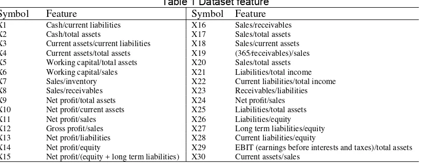
Dataset that is used in this study is dataset from Wieslaw [3]. The data is a result of an observation from 2 to 5 years on 120 companies. The dataset consists of 240 records (128 record are positive data dan the rest are negative data). Positive data means the companies are not bancrupt and the negative ones are the opposite. The features related to financial ratio. The features are described in Table 1.
Table 1 Dataset feature
Symbol Feature Symbol Feature
X1 Cash/current liabilities X16 Sales/receivables
X2 Cash/total assets X17 Sales/total assets
X3 Current assets/current liabilities X18 Sales/current assets
X4 Current assets/total assets X19 (365⁄receivables)/sales
X5 Working capital/total assets X20 Sales/total assets
X6 Working capital/sales X21 Liabilities/total income
X7 Sales/inventory X22 Current liabilities/total income
X8 Sales/receivables X23 Receivables/liabilities
X9 Net profit/total assets X24 Net profit/sales
X10 Net profit/current assets X25 Liabilities/total assets
X11 Net profit/sales X26 Liabilities/equity
X12 Gross profit/sales X27 Long term liabilities/equity
X13 Net profit/liabilities X28 Current liabilities/equity
X14 Net profit/equity X29 EBIT (earnings before interests and taxes)/total assets
X15 Net profit/(equity + long term liabilities) X30 Current assets/sales
3. Results and Analysis
In this comparative study, the performance of the cmpared methods is evaluated using k-fold cross validation. The k-fold cross validation a technique divide the dataset into training and testing set. With this technique, each record in dataset is used as testing data once and used as training data for k-1 times. The k value represent the fold number of the dataset. In this study, the fold number for k-NN, fuzzy k-NN, SVM and BNNSVM model is 5. And the fold number for MLR dan Hibrid of MLP+MLR is 4. The determination of these fold number is based on the best performnace that are achieved by the compared models.
The performance results of the compared models are represented as accuracy value. The accuracy metric is used because the number of positive and negative data is quite balance. The accuracy metric is defined in equation 19:
∗ % (19)
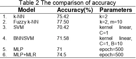
Table 2 The comparison of accuracy Model Accuracy(%) Parameters
1. k-NN 75.42 k=2
2. Fuzzy k-NN 77.50 k=2, m=10
3. SVM 70.42 kernel linear,
C=1
4. BNNSVM 71.58 kernel linear,
C=1, B=10
5. MLP 71 epoch=500
6. MLP+MLR 74.5 epoch=500
The second high accuracy is achieved by k-NN model with accuracy 75.42%. When compare to Fuzzy k-NN, this accuracy is lower than that of fuzzy k-NN accuracy. This describe that the membership degree of class affect the classification performance. The influence of the class membership function seems to reduce the noise effect which is generally occur in k-NN model. Therefore, the effect will lead the model to predict an appropriate class eventhough the difference between both class tendency is small.
The next high accuracy is 74.5% which is attained by MLP+MLR model. The accuracy of MLP+MLR is higher about 3.5% than that of original MLP model. The improvement of the accuracy shows that the linear characteristic that is calculated by MLR complement the non-linear characteristic that is exploited by MLP. The fuse of non-linear and non-non-linear characteristic indicate a positive contribution to the classification model performance.
The last result is reported for BNNSVM model. The performance of BNNSVM is not different compare to the performance of SVM model. The bagging process seems not provide advantage to the BNNSVM model. The possible explanation is because BNNSVM is more compatible when positive dataset and negative dataset is not balance. Meanwhile, the Bankruptcy dataset that is exploited for model building, has a balance proportion between positive and negative data.
4. Conclusion
Based on the comparison of accuracy from models that are build from k-NN, SVM dan MLP, it can be concluded that k-NN-based method is the most suitable method. Mainly, k-NN method that involve fuzzy logic. The fuzzy effect indicate the reduction of negative effect of noise. Therefore, for further research in Bankruptcy prediction model with features as listed in Table 1, an improvement model can be developed based on fuzzy k-NN method. Another suggestion is another advance k-NN-based method to be considered as model for Bankruptcy
References
[1] Tama B A, S Rodiyatul, Hermasyah H. An Early Detection Method of Type-2 Diabetes Mellitus in Public Hospital. Telkomnika vol 9 no 2 2011
[2] Nurmaini S, Tutuko B. A New Classification Technique in Mobile Robot Navigation. Telkomnika vol 9 no 3 2011.
[3] Wieslaw, P. Application of Discrete Predicting Structures in An Early Warning Expert System for Financial Distress. Tourism Management. 2004.
[4] Keller, J., Gray, M., & Givens, J. A Fuzzy k Nearest Neighbours Algorithm. IEEE Transaction on System, Man, and Cybernetics , SMC-15, 4. 1985.
[5] Chen, H. L., Yang, B., Wang, G., Liu, J., Xu, X., Wang, S.-J., et al. A Novel Bankruptcy Prediction Model Based on An Adaptive Fuzzy k-Nearest Neighbor Method. Knowledge-Based System , 24 (8), 1348-1359. (2011).
[6] Li, Hui and Sun, Ji. Forecasting Business Failure: The Use of Nearest-Neighbour Support Vectors and Correcting Imbalanced Samples - Evidence from Chinese Hotel Industry. 3, s.l. : Elsevier, Tourism Management, Vol. XXXIII, pp. 622-634. 2011.
[7] Khashei, Mehdi, Ali Zeinal Hamadani, and Mehdi Bijari. A novel hybrid classification model of ANN and MLR models. Expert Systems with Applications 39, 2011: 2606–2620.
[8] Tan, P. N., Steinbach, M., & Kumar, V. Introduction to Data Mining (4th ed.). Boston: Pearson Addison Wesley. 2006.