Jay L. Devore Probability and Statistics

(1)

(2)

(3)

(4)

Your First Study Break

www.CengageBrain.com

Get the best grade in the shortest time possible!

Now that you’ve bought the textbook . . .

Get a break on the study materials designed for your course! Visit CengageBrain.com and search for your textbook to find discounted print, digital and audio study tools that allow you to:

• Study in less time to get the grade you

want using online resources such as chapter quizzing, flashcards, and interactive study tools.

• Prepare for tests anywhere, anytime

• Practice, review, and master course

concepts using printed guides and manuals that work hand-in-hand with each chapter of your textbook.

(5)

(6)

Probability and Statistics

for Engineering

and the Sciences

JAY DEVORE

California Polytechnic State University, San Luis Obispo

(7)

(8)

(9)

Jay L. Devore

Editor in Chief: Michelle Julet Publisher: Richard Stratton

Senior Sponsoring Editor: Molly Taylor Senior Development Editor: Jay Campbell Senior Editorial Assistant: Shaylin Walsh Media Editor: Andrew Coppola Marketing Manager: Ashley Pickering Marketing Communications Manager: Mary

Anne Payumo

Content Project Manager: Cathy Brooks Art Director: Linda Helcher

Print Buyer: Diane Gibbons

Rights Acquisition Specialists: Image: Mandy Groszko; Text: Katie Huha

Production Service: Elm Street Publishing Services

Text Designer: Diane Beasley Cover Designer: Rokusek Design

ALL RIGHTS RESERVED. No part of this work covered by the copyright herein may be reproduced, transmitted, stored, or used in any form or by any means graphic, electronic, or mechanical, including but not limited to photocopying, recording, scanning, digitizing, taping, Web distribution, information networks, or information storage and retrieval systems, except as permitted under Section 107 or 108 of the 1976 United States Copyright Act, without the prior written permission of the publisher.

Printed in the United States of America 1 2 3 4 5 6 7 14 13 12 11 10

For product information and technology assistance, contact us at

Cengage Learning Customer & Sales Support, 1-800-354-9706 For permission to use material from this text or product, submit all requests online at www.cengage.com/permissions.

Further permissions questions can be emailed to

permissionrequest@cengage.com.

Library of Congress Control Number: 2010927429

ISBN-13: 978-0-538-73352-6 ISBN-10: 0-538-73352-7

Brooks/Cole

20Channel Center Street Boston, MA 02210 USA

Cengage Learning is a leading provider of customized learning solutions with office locations around the globe, including Singapore, the United Kingdom, Australia, Mexico, Brazil, and Japan. Locate your local office at

international.cengage.com/region

Cengage Learning products are represented in Canada by Nelson Education, Ltd.

For your course and learning solutions, visit www.cengage.com.

(10)

v

Philip, who is highly

(11)

(12)

vii

Discrete Random Variables

(13)

Introduction 137

4.1 Probability Density Functions 138

4.2 Cumulative Distribution Functions and Expected Values 143 4.3 The Normal Distribution 152

4.4 The Exponential and Gamma Distributions 165 4.5 Other Continuous Distributions 171

4.6 Probability Plots 178

Introduction 193

5.1 Jointly Distributed Random Variables 194

5.2 Expected Values, Covariance, and Correlation 206 5.3 Statistics and Their Distributions 212

5.4 The Distribution of the Sample Mean 223 5.5 The Distribution of a Linear Combination 230

6

Point Estimation

7

Statistical Intervals Based on a Single Sample

Introduction 239

6.1 Some General Concepts of Point Estimation 240 6.2 Methods of Point Estimation 255

Introduction 267

7.1 Basic Properties of Confidence Intervals 268

7.2 Large-Sample Confidence Intervals for a Population Mean and Proportion 276

4

Continuous Random Variables

and Probability Distributions

5

Joint Probability Distributions

(14)

7.3 Intervals Based on a Normal Population Distribution 285 7.4 Confidence Intervals for the Variance and Standard Deviation

of a Normal Population 294 Supplementary Exercises 297 Bibliography 299

8

Tests of Hypotheses Based on a Single Sample

Introduction 300

8.1 Hypotheses and Test Procedures 301 8.2 Tests About a Population Mean 310

8.3 Tests Concerning a Population Proportion 323 8.4 P-Values 328

8.5 Some Comments on Selecting a Test 339 Supplementary Exercises 342

Bibliography 344

9

Inferences Based on Two Samples

Introduction 345

9.1 zTests and Confidence Intervals for a Difference Between Two Population Means 346

9.2 The Two-Sample tTest and Confidence Interval 357 9.3 Analysis of Paired Data 365

9.4 Inferences Concerning a Difference Between Population Proportions 375 9.5 Inferences Concerning Two Population Variances 382

10

The Analysis of Variance

Introduction 391

10.1 Single-Factor ANOVA 392

10.2 Multiple Comparisons in ANOVA 402 10.3 More on Single-Factor ANOVA 408

(15)

11

Multifactor Analysis of Variance

Introduction 419

11.1 Two-Factor ANOVA with K_ij1 420 11.2 Two-Factor ANOVA with K_ij1 433 11.3 Three-Factor ANOVA 442

11.4 2p_{Factorial Experiments 451}

12

Simple Linear Regression and Correlation

Introduction 468

12.1 The Simple Linear Regression Model 469 12.2 Estimating Model Parameters 477

12.3 Inferences About the Slope Parameter ␤₁ 490 12.4 Inferences Concerning and the Prediction

of Future YValues 499 12.5 Correlation 508

mY#x*

13

Nonlinear and Multiple Regression

Introduction 523

13.1 Assessing Model Adequacy 524

13.2 Regression with Transformed Variables 531 13.3 Polynomial Regression 543

13.4 Multiple Regression Analysis 553 13.5 Other Issues in Multiple Regression 574

14

Goodness-of-Fit Tests and Categorical Data Analysis

Introduction 594

(16)

14.2 Goodness-of-Fit Tests for Composite Hypotheses 602 14.3 Two-Way Contingency Tables 613

15

Distribution-Free Procedures

Introduction 625

15.1 The Wilcoxon Signed-Rank Test 626 15.2 The Wilcoxon Rank-Sum Test 634

15.3 Distribution-Free Confidence Intervals 640 15.4 Distribution-Free ANOVA 645

16

Quality Control Methods

Introduction 651

16.1 General Comments on Control Charts 652 16.2 Control Charts for Process Location 654 16.3 Control Charts for Process Variation 663 16.4 Control Charts for Attributes 668 16.5 CUSUM Procedures 672

16.6 Acceptance Sampling 680 Supplementary Exercises 686 Bibliography 687

Appendix Tables

A.1 Cumulative Binomial Probabilities A-2 A.2 Cumulative Poisson Probabilities A-4 A.3 Standard Normal Curve Areas A-6 A.4 The Incomplete Gamma Function A-8 A.5 Critical Values for tDistributions A-9

A.6 Tolerance Critical Values for Normal Population Distributions A-10 A.7 Critical Values for Chi-Squared Distributions A-11

A.8 tCurve Tail Areas A-12

A.9 Critical Values for FDistributions A-14

(17)

A.11 Chi-Squared Curve Tail Areas A-21

A.12 Critical Values for the Ryan-Joiner Test of Normality A-23 A.13 Critical Values for the Wilcoxon Signed-Rank Test A-24 A.14 Critical Values for the Wilcoxon Rank-Sum Test A-25 A.15 Critical Values for the Wilcoxon Signed-Rank Interval A-26 A.16 Critical Values for the Wilcoxon Rank-Sum Interval A-27 A.17 ␤Curves for tTests A-28

Answers to Selected Odd-Numbered Exercises A-29 Glossary of Symbols /Abbreviations G-1

(18)

xiii

Preface

Purpose

The use of probability models and statistical methods for analyzing data has become common practice in virtually all scientific disciplines. This book attempts to provide a comprehensive introduction to those models and methods most likely to be encoun-tered and used by students in their careers in engineering and the natural sciences. Although the examples and exercises have been designed with scientists and engi-neers in mind, most of the methods covered are basic to statistical analyses in many other disciplines, so that students of business and the social sciences will also profit from reading the book.

Approach

Students in a statistics course designed to serve other majors may be initially skeptical of the value and relevance of the subject matter, but my experience is that students canbe

turned on to statistics by the use of good examples and exercises that blend their every-day experiences with their scientific interests. Consequently, I have worked hard to find examples of real, rather than artificial, data—data that someone thought was worth col-lecting and analyzing. Many of the methods presented, especially in the later chapters on statistical inference, are illustrated by analyzing data taken from published sources, and many of the exercises also involve working with such data. Sometimes the reader may be unfamiliar with the context of a particular problem (as indeed I often was), but I have found that students are more attracted by real problems with a somewhat strange context than by patently artificial problems in a familiar setting.

Mathematical Level

The exposition is relatively modest in terms of mathematical development. Substantial use of the calculus is made only in Chapter 4 and parts of Chapters 5 and 6. In particu-lar, with the exception of an occasional remark or aside, calculus appears in the inference part of the book only—in the second section of Chapter 6. Matrix algebra is not used at all. Thus almost all the exposition should be accessible to those whose mathematical background includes one semester or two quarters of differential and integral calculus.

Content

(19)

returns for an extensive encore in Chapter 13. The last three chapters develop chi-squared methods, distribution-free (nonparametric) procedures, and techniques from statistical quality control.

Helping Students Learn

Although the book’s mathematical level should give most science and engineering students little difficulty, working toward an understanding of the concepts and gain-ing an appreciation for the logical development of the methodology may sometimes require substantial effort. To help students gain such an understanding and appreci-ation, I have provided numerous exercises ranging in difficulty from many that involve routine application of text material to some that ask the reader to extend con-cepts discussed in the text to somewhat new situations. There are many more exer-cises than most instructors would want to assign during any particular course, but I recommend that students be required to work a substantial number of them; in a problem-solving discipline, active involvement of this sort is the surest way to iden-tify and close the gaps in understanding that inevitably arise. Answers to most odd-numbered exercises appear in the answer section at the back of the text. In addition, a Student Solutions Manual, consisting of worked-out solutions to virtually all the odd-numbered exercises, is available.

To access additional course materials and companion resources, please visit www.cengagebrain.com. At the CengageBrain.com home page, search for the ISBN of your title (from the back cover of your book) using the search box at the top of the page. This will take you to the product page where free companion resources can be found.

New for This Edition

• A Glossary of Symbols/Abbreviations appears at the end of the book (the author apologizes for his laziness in not getting this together for earlier editions!) and a small set of sample exams appears on the companion website (available at www.cengage.com/login).

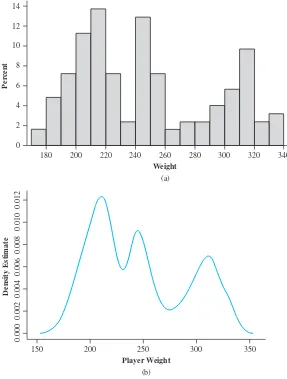
• Many new examples and exercises, almost all based on real data or actual prob-lems. Some of these scenarios are less technical or broader in scope than what has been included in previous editions—for example, weights of football players (to illustrate multimodality), fundraising expenses for charitable organizations, and the comparison of grade point averages for classes taught by part-time faculty with those for classes taught by full-time faculty.

• The material on P-values has been substantially rewritten. The P-value is now

ini-tially defined as a probability rather than as the smallest significance level for which the null hypothesis can be rejected. A simulation experiment is presented to illustrate the behavior of P-values.

• Chapter 1 contains a new subsection on “The Scope of Modern Statistics” to indicate how statisticians continue to develop new methodology while working on problems in a wide spectrum of disciplines.

(20)

Acknowledgments

My colleagues at Cal Poly have provided me with invaluable support and feedback over the years. I am also grateful to the many users of previous editions who have made suggestions for improvement (and on occasion identified errors). A special note of thanks goes to Matt Carlton for his work on the two solutions manuals, one for instructors and the other for students.

(21)

Paul J. Smith, University of Maryland; Richard M. Soland, The George Washington University; Clifford Spiegelman, Texas A & M University; Jery Stedinger, Cornell University; David Steinberg, Tel Aviv University; William Thistleton, State University of New York Institute of Technology; G. Geoffrey Vining, University of Florida; Bhutan Wadhwa, Cleveland State University; Gary Wasserman, Wayne State University; Elaine Wenderholm, State University of New York–Oswego; Samuel P. Wilcock, Messiah College; Michael G. Zabetakis, University of Pittsburgh; and Maria Zack, Point Loma Nazarene University.

Danielle Urban of Elm Street Publishing Services has done a terrific job of supervising the book's production. Once again I am compelled to express my grat-itude to all those people at Cengage who have made important contributions over the course of my textbook writing career. For this most recent edition, special thanks go to Jay Campbell (for his timely and informed feedback throughout the project), Molly Taylor, Shaylin Walsh, Ashley Pickering, Cathy Brooks, and Andrew Coppola. I also greatly appreciate the stellar work of all those Cengage Learning sales representatives who have labored to make my books more visible to the statistical community. Last but by no means least, a heartfelt thanks to my wife Carol for her decades of support, and to my daughters for providing inspiration through their own achievements.

(22)

1

Overview and Descriptive

Statistics

“I am not much given to regret, so I puzzled over this one a while. Should have taken much more statistics in college, I think.”

—Max Levchin, Paypal Co-founder, Slide Founder

Quote of the week from the Web site of the

American Statistical Association on November 23, 2010

“I keep saying that the sexy job in the next 10 years will be statisticians, and I’m not kidding.”

—Hal Varian, Chief Economist at Google

August 6, 2009, The New York Times

INTRODUCTION

Statistical concepts and methods are not only useful but indeed often indis-pensable in understanding the world around us. They provide ways of gaining new insights into the behavior of many phenomena that you will encounter in your chosen field of specialization in engineering or science.

(23)

Vehicle Emissions Variability” (J. of the Air and Waste Mgmt. Assoc., 1996: 667–675), the acceptance of the FTP as a gold standard has led to the widespread belief that repeated measurements on the same vehicle would yield identical (or nearly identical) results. The authors of the article applied the FTP to seven vehicles characterized as “high emitters.” Here are the results for one such vehicle:

HC (gm/mile) 13.8 18.3 32.2 32.5 CO (gm/mile) 118 149 232 236

The substantial variation in both the HC and CO measurements casts consider-able doubt on conventional wisdom and makes it much more difficult to make precise assessments about emissions levels.

How can statistical techniques be used to gather information and draw conclusions? Suppose, for example, that a materials engineer has developed a coating for retarding corrosion in metal pipe under specified circumstances. If this coating is applied to different segments of pipe, variation in environmental conditions and in the segments themselves will result in more substantial cor-rosion on some segments than on others. Methods of statistical analysis could be used on data from such an experiment to decide whether the average amount of corrosion exceeds an upper specification limit of some sort or to pre-dict how much corrosion will occur on a single piece of pipe.

Alternatively, suppose the engineer has developed the coating in the belief that it will be superior to the currently used coating. A comparative experiment could be carried out to investigate this issue by applying the current coating to some segments of pipe and the new coating to other segments. This must be done with care lest the wrong conclusion emerge. For example, perhaps the aver-age amount of corrosion is identical for the two coatings. However, the new coating may be applied to segments that have superior ability to resist corrosion and under less stressful environmental conditions compared to the segments and conditions for the current coating. The investigator would then likely observe a difference between the two coatings attributable not to the coatings themselves, but just to extraneous variation. Statistics offers not only methods for analyzing the results of experiments once they have been carried out but also suggestions for how experiments can be performed in an efficient manner to mitigate the effects of variation and have a better chance of producing correct conclusions.

1.1

Populations, Samples, and Processes

(24)

An investigation will typically focus on a well-defined collection of objects constituting a populationof interest. In one study, the population might consist of all gelatin capsules of a particular type produced during a specified period. Another investigation might involve the population consisting of all individuals who received a B.S. in engineering during the most recent academic year. When desired informa-tion is available for all objects in the populainforma-tion, we have what is called a census. Constraints on time, money, and other scarce resources usually make a census impractical or infeasible. Instead, a subset of the population—a sample—is selected in some prescribed manner. Thus we might obtain a sample of bearings from a par-ticular production run as a basis for investigating whether bearings are conforming to manufacturing specifications, or we might select a sample of last year’s engineer-ing graduates to obtain feedback about the quality of the engineerengineer-ing curricula.

We are usually interested only in certain characteristics of the objects in a pop-ulation: the number of flaws on the surface of each casing, the thickness of each cap-sule wall, the gender of an engineering graduate, the age at which the individual graduated, and so on. A characteristic may be categorical, such as gender or type of malfunction, or it may be numerical in nature. In the former case, the valueof the

characteristic is a category (e.g., female or insufficient solder), whereas in the latter

case, the value is a number (e.g., or ). A variable

is any characteristic whose value may change from one object to another in the population. We shall initially denote variables by lowercase letters from the end of our alphabet. Examples include

Data results from making observations either on a single variable or simultaneously on two or more variables. A univariatedata set consists of observations on a single variable. For example, we might determine the type of transmission, automatic (A) or manual (M), on each of ten automobiles recently purchased at a certain dealer-ship, resulting in the categorical data set

The following sample of lifetimes (hours) of brand D batteries put to a certain use is a numerical univariate data set:

We have bivariatedata when observations are made on each of two variables. Our data set might consist of a (height, weight) pair for each basketball player on a team, with the first observation as (72, 168), the second as (75, 212), and so on. If

an engineer determines the value of both and

for component failure, the resulting data set is bivariate with one variable numeri-cal and the other categorinumeri-cal. Multivariatedata arises when observations are made on more than one variable (so bivariate is a special case of multivariate). For exam-ple, a research physician might determine the systolic blood pressure, diastolic blood pressure, and serum cholesterol level for each patient participating in a study. Each observation would be a triple of numbers, such as (120, 80, 146). In many multivariate data sets, some variables are numerical and others are categorical. Thus the annual automobile issue of Consumer Reportsgives values of such variables as

type of vehicle (small, sporty, compact, mid-size, large), city fuel efficiency (mpg), highway fuel efficiency (mpg), drivetrain type (rear wheel, front wheel, four wheel), and so on.

y5 reason

x5 component lifetime 5.6 5.1 6.2 6.0 5.8 6.5 5.8 5.5

M A A A M A A M A A

z5 braking distance of an automobile under specified conditions

y5 _{number of visits to a particular Web site during a specified period}

x5 brand of calculator owned by a student

(25)

Example 1.1

Branches of Statistics

An investigator who has collected data may wish simply to summarize and describe important features of the data. This entails using methods from descriptive statistics. Some of these methods are graphical in nature; the construction of histograms, boxplots, and scatter plots are primary examples. Other descriptive methods involve calculation of numerical summary measures, such as means, standard deviations, and correlation coefficients. The wide availability of statistical computer software packages has made these tasks much easier to carry out than they used to be. Computers are much more efficient than human beings at calculation and the creation of pictures (once they have received appropriate instructions from the user!). This means that the investigator doesn’t have to expend much effort on “grunt work” and will have more time to study the data and extract important messages. Throughout this book, we will present output from various packages such as Minitab, SAS, S-Plus, and R. The R software can be downloaded without charge from the site http://www.r-project.org.

Charity is a big business in the United States. The Web site charitynavigator.com gives information on roughly 5500 charitable organizations, and there are many smaller charities that fly below the navigator’s radar screen. Some charities operate very efficiently, with fundraising and administrative expenses that are only a small percentage of total expenses, whereas others spend a high percentage of what they take in on such activities. Here is data on fundraising expenses as a percentage of total expenditures for a random sample of 60 charities:

6.1 12.6 34.7 1.6 18.8 2.2 3.0 2.2 5.6 3.8

2.2 3.1 1.3 1.1 14.1 4.0 21.0 6.1 1.3 20.4

7.5 3.9 10.1 8.1 19.5 5.2 12.0 15.8 10.4 5.2 6.4 10.8 83.1 3.6 6.2 6.3 16.3 12.7 1.3 0.8

8.8 5.1 3.7 26.3 6.0 48.0 8.2 11.7 7.2 3.9

15.3 16.6 8.8 12.0 4.7 14.7 6.4 17.0 2.5 16.2

Without any organization, it is difficult to get a sense of the data’s most prominent features—what a typical (i.e. representative) value might be, whether values are highly concentrated about a typical value or quite dispersed, whether there are any

0 0 10 20

Fr

equency

30 40 Stem–and–leaf of FundRsng N = 60 Leaf Unit = 1.0

0 0111112222333333344 0 55556666666778888 1 0001222244 1 55666789 2 01 2 6 3 3 4 4 8 5 5 6 6 7 7 8 3

4

10 20 30 40 50

FundRsng

60 70 80 90

(26)

Example 1.2

gaps in the data, what fraction of the values are less than 20%, and so on. Figure 1.1 shows what is called a stem-and-leaf displayas well as a histogram.In Section 1.2

we will discuss construction and interpretation of these data summaries. For the moment, we hope you see how they begin to describe how the percentages are dis-tributed over the range of possible values from 0 to 100. Clearly a substantial major-ity of the charities in the sample spend less than 20% on fundraising, and only a few percentages might be viewed as beyond the bounds of sensible practice. ■

Having obtained a sample from a population, an investigator would frequently like to use sample information to draw some type of conclusion (make an inference of some sort) about the population. That is, the sample is a means to an end rather than an end in itself. Techniques for generalizing from a sample to a population are gathered within the branch of our discipline called inferential statistics.

Material strength investigations provide a rich area of application for statistical meth-ods. The article “Effects of Aggregates and Microfillers on the Flexural Properties of Concrete” (Magazine of Concrete Research, 1997: 81–98) reported on a study of

strength properties of high-performance concrete obtained by using superplasticizers and certain binders. The compressive strength of such concrete had previously been investigated, but not much was known about flexural strength (a measure of ability to resist failure in bending). The accompanying data on flexural strength (in

MegaPascal, MPa, where ) appeared in the article

cited:

5.9 7.2 7.3 6.3 8.1 6.8 7.0 7.6 6.8 6.5 7.0 6.3 7.9 9.0 8.2 8.7 7.8 9.7 7.4 7.7 9.7 7.8 7.7 11.6 11.3 11.8 10.7 Suppose we want an estimateof the average value of flexural strength for all beams

that could be made in this way (if we conceptualize a population of all such beams, we are trying to estimate the population mean). It can be shown that, with a high degree of confidence, the population mean strength is between 7.48 MPa and 8.80 MPa; we call this a confidence intervalor interval estimate.Alternatively, this

data could be used to predict the flexural strength of a singlebeam of this type. With

a high degree of confidence, the strength of a single such beam will exceed 7.35 MPa; the number 7.35 is called a lower prediction bound. ■ The main focus of this book is on presenting and illustrating methods of ential statistics that are useful in scientific work. The most important types of infer-ential procedures—point estimation, hypothesis testing, and estimation by confidence intervals—are introduced in Chapters 6–8 and then used in more com-plicated settings in Chapters 9–16. The remainder of this chapter presents methods from descriptive statistics that are most used in the development of inference.

Chapters 2–5 present material from the discipline of probability. This material ultimately forms a bridge between the descriptive and inferential techniques. Mastery of probability leads to a better understanding of how inferential procedures are developed and used, how statistical conclusions can be translated into everyday language and interpreted, and when and where pitfalls can occur in applying the methods. Probability and statistics both deal with questions involving populations and samples, but do so in an “inverse manner” to one another.

In a probability problem, properties of the population under study are assumed known (e.g., in a numerical population, some specified distribution of the population values may be assumed), and questions regarding a sample taken from the population are posed and answered. In a statistics problem, characteristics of a

(27)

Example 1.3

sample are available to the experimenter, and this information enables the experi-menter to draw conclusions about the population. The relationship between the two disciplines can be summarized by saying that probability reasons from the population to the sample (deductive reasoning), whereas inferential statistics rea-sons from the sample to the population (inductive reasoning). This is illustrated in Figure 1.2.

Before we can understand what a particular sample can tell us about the pop-ulation, we should first understand the uncertainty associated with taking a sample from a given population. This is why we study probability before statistics.

As an example of the contrasting focus of probability and inferential statistics, con-sider drivers’ use of manual lap belts in cars equipped with automatic shoulder belt systems. (The article “Automobile Seat Belts: Usage Patterns in Automatic Belt Systems,” Human Factors,1998: 126–135, summarizes usage data.) In probability,

we might assume that 50% of all drivers of cars equipped in this way in a certain metropolitan area regularly use their lap belt (an assumption about the population), so we might ask, “How likely is it that a sample of 100 such drivers will include at least 70 who regularly use their lap belt?” or “How many of the drivers in a sample of size 100 can we expect to regularly use their lap belt?” On the other hand, in infer-ential statistics, we have sample information available; for example, a sample of 100 drivers of such cars revealed that 65 regularly use their lap belt. We might then ask, “Does this provide substantial evidence for concluding that more than 50% of all such drivers in this area regularly use their lap belt?” In this latter scenario, we are attempting to use sample information to answer a question about the structure of the

entire population from which the sample was selected. _■

In the foregoing lap belt example, the population is well defined and concrete: all drivers of cars equipped in a certain way in a particular metropolitan area. In Example 1.2, however, the strength measurements came from a sample of prototype beams that had not been selected from an existing population. Instead, it is conven-ient to think of the population as consisting of all possible strength measurements that might be made under similar experimental conditions. Such a population is referred to as a conceptualor hypothetical population.There are a number of prob-lem situations in which we fit questions into the framework of inferential statistics by conceptualizing a population.

The Scope of Modern Statistics

These days statistical methodology is employed by investigators in virtually all dis-ciplines, including such areas as

• molecular biology (analysis of microarray data)

• ecology (describing quantitatively how individuals in various animal and plant populations are spatially distributed)

Population

Probability

Inferential statistics

Sample

(28)

• materials engineering (studying properties of various treatments to retard corrosion)

• marketing (developing market surveys and strategies for marketing new products)

• public health (identifying sources of diseases and ways to treat them)

• civil engineering (assessing the effects of stress on structural elements and the impacts of traffic flows on communities)

As you progress through the book, you’ll encounter a wide spectrum of different sce-narios in the examples and exercises that illustrate the application of techniques from probability and statistics. Many of these scenarios involve data or other material extracted from articles in engineering and science journals. The methods presented herein have become established and trusted tools in the arsenal of those who work with data. Meanwhile, statisticians continue to develop new models for describing random-ness, and uncertainty and new methodology for analyzing data. As evidence of the con-tinuing creative efforts in the statistical community, here are titles and capsule descriptions of some articles that have recently appeared in statistics journals (Journal of the American Statistical Associationis abbreviated JASA, and AASis short for the Annals of Applied Statistics,two of the many prominent journals in the discipline):

• “Modeling Spatiotemporal Forest Health Monitoring Data” (JASA,2009:

899–911): Forest health monitoring systems were set up across Europe in the 1980s in response to concerns about air-pollution-related forest dieback, and have continued operation with a more recent focus on threats from climate change and increased ozone levels. The authors develop a quantitative descrip-tion of tree crown defoliadescrip-tion, an indicator of tree health.

• “Active Learning Through Sequential Design, with Applications to the Detection of Money Laundering” (JASA,2009: 969–981): Money laundering involves

con-cealing the origin of funds obtained through illegal activities. The huge number of transactions occurring daily at financial institutions makes detection of money laundering difficult. The standard approach has been to extract various summary quantities from the transaction history and conduct a time-consuming investiga-tion of suspicious activities. The article proposes a more efficient statistical method and illustrates its use in a case study.

• “Robust Internal Benchmarking and False Discovery Rates for Detecting Racial Bias in Police Stops” (JASA,2009: 661–668): Allegations of police actions that

are attributable at least in part to racial bias have become a contentious issue in many communities. This article proposes a new method that is designed to reduce the risk of flagging a substantial number of “false positives” (individuals falsely identified as manifesting bias). The method was applied to data on 500,000 pedestrian stops in New York City in 2006; of the 3000 officers regu-larly involved in pedestrian stops, 15 were identified as having stopped a sub-stantially greater fraction of Black and Hispanic people than what would be predicted were bias absent.

• “Records in Athletics Through Extreme Value Theory” (JASA,2008:

(29)

men’s marathon record, but that the current women’s marathon record is almost 5 minutes longer than what can ultimately be achieved. The methodology also has applications to such issues as ensuring airport runways are long enough and that dikes in Holland are high enough.

• “Analysis of Episodic Data with Application to Recurrent Pulmonary

Exacerbations in Cystic Fibrosis Patients” (JASA,2008: 498–510): The analysis

of recurrent medical events such as migraine headaches should take into account not only when such events first occur but also how long they last—length of episodes may contain important information about the severity of the disease or malady, associated medical costs, and the quality of life. The article proposes a technique that summarizes both episode frequency and length of episodes, and allows effects of characteristics that cause episode occurrence to vary over time. The technique is applied to data on cystic fibrosis patients (CF is a serious genetic disorder affecting sweat and other glands).

• “Prediction of Remaining Life of Power Transformers Based on Left Truncated and Right Censored Lifetime Data” (AAS,2009: 857–879): There are roughly

150,000 high-voltage power transmission transformers in the United States. Unexpected failures can cause substantial economic losses, so it is important to have predictions for remaining lifetimes. Relevant data can be complicated because lifetimes of some transformers extend over several decades during which records were not necessarily complete. In particular, the authors of the article use data from a certain energy company that began keeping careful records in 1980. But some transformers had been installed before January 1, 1980, and were still in service after that date (“left truncated” data), whereas other units were still in serv-ice at the time of the investigation, so their complete lifetimes are not available (“right censored” data). The article describes various procedures for obtaining an interval of plausible values (a prediction interval) for a remaining lifetime and for

the cumulative number of failures over a specified time period.

• “The BARISTA: A Model for Bid Arrivals in Online Auctions” (AAS,2007:

412–441): Online auctions such as those on eBay and uBid often have character-istics that differentiate them from traditional auctions. One particularly important difference is that the number of bidders at the outset of many traditional auctions is fixed, whereas in online auctions this number and the number of resulting bids are not predetermined. The article proposes a new BARISTA (for Bid ARivals In STAges) model for describing the way in which bids arrive online. The model allows for higher bidding intensity at the outset of the auction and also as the auction comes to a close. Various properties of the model are investigated and then validated using data from eBay.com on auctions for Palm M515 personal assistants, Microsoft Xbox games, and Cartier watches.

• “Statistical Challenges in the Analysis of Cosmic Microwave Background Radiation” (AAS,2009: 61–95): The cosmic microwave background (CMB) is a

significant source of information about the early history of the universe. Its radi-ation level is uniform, so extremely delicate instruments have been developed to measure fluctuations. The authors provide a review of statistical issues with CMB data analysis; they also give many examples of the application of statistical procedures to data obtained from a recent NASA satellite mission, the Wilkinson Microwave Anisotropy Probe.

(30)

Nov. 23, 2009, New York Timesreported in an article “Behind Cancer Guidelines,

Quest for Data” that the new science for cancer investigations and more sophisti-cated methods for data analysis spurred the U.S. Preventive Services task force to re-examine guidelines for how frequently middle-aged and older women should have mammograms. The panel commissioned six independent groups to do statis-tical modeling. The result was a new set of conclusions, including an assertion that mammograms every two years are nearly as beneficial to patients as annual mam-mograms, but confer only half the risk of harms. Donald Berry, a very prominent biostatistician, was quoted as saying he was pleasantly surprised that the task force took the new research to heart in making its recommendations. The task force’s report has generated much controversy among cancer organizations, politicians, and women themselves.

It is our hope that you will become increasingly convinced of the importance and relevance of the discipline of statistics as you dig more deeply into the book and the subject. Hopefully you’ll be turned on enough to want to continue your statisti-cal education beyond your current course.

Enumerative Versus Analytic Studies

W. E. Deming, a very influential American statistician who was a moving force in Japan’s quality revolution during the 1950s and 1960s, introduced the distinction between enumerative studiesand analytic studies.In the former, interest is focused

on a finite, identifiable, unchanging collection of individuals or objects that make up a population. A sampling frame—that is, a listing of the individuals or objects

to be sampled—is either available to an investigator or else can be constructed. For example, the frame might consist of all signatures on a petition to qualify a certain initiative for the ballot in an upcoming election; a sample is usually selected to ascertain whether the number of valid signatures exceeds a specified value. As

another example, the frame may contain serial numbers of all furnaces manufac-tured by a particular company during a certain time period; a sample may be selected to infer something about the average lifetime of these units. The use of inferential methods to be developed in this book is reasonably noncontroversial in such settings (though statisticians may still argue over which particular methods should be used).

An analytic study is broadly defined as one that is not enumerative in nature. Such studies are often carried out with the objective of improving a future product by taking action on a process of some sort (e.g., recalibrating equipment or adjusting the level of some input such as the amount of a catalyst). Data can often be obtained only on an existing process, one that may differ in important respects from the future process. There is thus no sampling frame listing the indi-viduals or objects of interest. For example, a sample of five turbines with a new design may be experimentally manufactured and tested to investigate efficiency. These five could be viewed as a sample from the conceptual population of all pro-totypes that could be manufactured under similar conditions, but notnecessarily

as representative of the population of units manufactured once regular production gets underway. Methods for using sample information to draw conclusions about future production units may be problematic. Someone with expertise in the area of turbine design and engineering (or whatever other subject area is relevant) should be called upon to judge whether such extrapolation is sensible. A good exposition of these issues is contained in the article “Assumptions for Statistical Inference” by Gerald Hahn and William Meeker (The American Statistician,

(31)

Example 1.4

Collecting Data

Statistics deals not only with the organization and analysis of data once it has been collected but also with the development of techniques for collecting the data. If data is not properly collected, an investigator may not be able to answer the questions under consideration with a reasonable degree of confidence. One common problem is that the target population—the one about which conclusions are to be drawn—may be different from the population actually sampled. For example, advertisers would like various kinds of information about the television-viewing habits of potential cus-tomers. The most systematic information of this sort comes from placing monitoring devices in a small number of homes across the United States. It has been conjectured that placement of such devices in and of itself alters viewing behavior, so that char-acteristics of the sample may be different from those of the target population.

When data collection entails selecting individuals or objects from a frame, the simplest method for ensuring a representative selection is to take a simple random sample.This is one for which any particular subset of the specified size (e.g., a

sam-ple of size 100) has the same chance of being selected. For examsam-ple, if the frame consists of 1,000,000 serial numbers, the numbers 1, 2, . . . , up to 1,000,000 could be placed on identical slips of paper. After placing these slips in a box and thor-oughly mixing, slips could be drawn one by one until the requisite sample size has been obtained. Alternatively (and much to be preferred), a table of random numbers or a computer’s random number generator could be employed.

Sometimes alternative sampling methods can be used to make the selection process easier, to obtain extra information, or to increase the degree of confidence in conclusions. One such method, stratified sampling,entails separating the population

units into nonoverlapping groups and taking a sample from each one. For example, a manufacturer of DVD players might want information about customer satisfaction for units produced during the previous year. If three different models were manu-factured and sold, a separate sample could be selected from each of the three corre-sponding strata. This would result in information on all three models and ensure that no one model was over- or underrepresented in the entire sample.

Frequently a “convenience” sample is obtained by selecting individuals or objects without systematic randomization. As an example, a collection of bricks may be stacked in such a way that it is extremely difficult for those in the center to be selected. If the bricks on the top and sides of the stack were somehow different from the others, resulting sample data would not be representative of the population. Often an investigator will assume that such a convenience sample approximates a random sample, in which case a statistician’s repertoire of inferential methods can be used; however, this is a judgment call. Most of the methods discussed herein are based on a variation of simple random sampling described in Chapter 5.

Engineers and scientists often collect data by carrying out some sort of designed experiment. This may involve deciding how to allocate several different treatments (such as fertilizers or coatings for corrosion protection) to the various experimental units (plots of land or pieces of pipe). Alternatively, an investigator may systematically vary the levels or categories of certain factors (e.g., pressure or type of insulating material) and observe the effect on some response variable (such as yield from a production process).

An article in the New York Times (Jan. 27, 1987) reported that heart attack risk

(32)

Example 1.5

according to a specified regimen. Subjects were randomly assigned to the groups to protect against any biases and so that probability-based methods could be used to analyze the data. Of the 11,034 individuals in the control group, 189 subsequently experienced heart attacks, whereas only 104 of the 11,037 in the aspirin group had a heart attack. The incidence rate of heart attacks in the treatment group was only about half that in the control group. One possible explanation for this result is chance variation—that aspirin really doesn’t have the desired effect and the observed dif-ference is just typical variation in the same way that tossing two identical coins would usually produce different numbers of heads. However, in this case, inferential methods suggest that chance variation by itself cannot adequately explain the

mag-nitude of the observed difference. ■

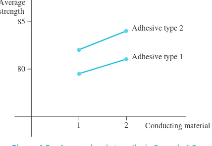
An engineer wishes to investigate the effects of both adhesive type and conductor material on bond strength when mounting an integrated circuit (IC) on a certain sub-strate. Two adhesive types and two conductor materials are under consideration. Two observations are made for each adhesive-type/conductor-material combination, resulting in the accompanying data:

Adhesive Type Conductor Material Observed Bond Strength Average

1 1 82, 77 79.5

1 2 75, 87 81.0

2 1 84, 80 82.0

2 2 78, 90 84.0

Conducting material Average

strength

1 2

80 85

Adhesive type 2

[image:32.576.279.493.446.594.2]

Adhesive type 1

Figure 1.3 Average bond strengths in Example 1.5

The resulting average bond strengths are pictured in Figure 1.3. It appears that adhe-sive type 2 improves bond strength as compared with type 1 by about the same amount whichever one of the conducting materials is used, with the 2, 2 combina-tion being best. Inferential methods can again be used to judge whether these effects are real or simply due to chance variation.

Suppose additionally that there are two cure times under consideration and also two types of IC post coating. There are then combinations of these four factors, and our engineer may not have enough resources to make even a single obser-vation for each of these combinations. In Chapter 11, we will see how the careful selec-tion of a fracselec-tion of these possibilities will usually yield the desired informaselec-tion. _■

(33)

EXERCISES

Section 1.1 (1–9)

1. Give one possible sample of size 4 from each of the

follow-ing populations:

a. All daily newspapers published in the United States b. All companies listed on the New York Stock Exchange c. All students at your college or university

d. All grade point averages of students at your college or

university

2. For each of the following hypothetical populations, give a

plausible sample of size 4:

a. All distances that might result when you throw a football b. Page lengths of books published 5 years from now c. All possible earthquake-strength measurements (Richter

scale) that might be recorded in California during the next year

d. All possible yields (in grams) from a certain chemical

reaction carried out in a laboratory

3. Consider the population consisting of all computers of a

cer-tain brand and model, and focus on whether a computer needs service while under warranty.

a. Pose several probability questions based on selecting a

sample of 100 such computers.

b. What inferential statistics question might be answered by

determining the number of such computers in a sample of size 100 that need warranty service?

4. a. Give three different examples of concrete populations and

three different examples of hypothetical populations.

b. For one each of your concrete and your hypothetical

pop-ulations, give an example of a probability question and an example of an inferential statistics question.

5. Many universities and colleges have instituted supplemental

instruction (SI) programs, in which a student facilitator meets regularly with a small group of students enrolled in the course to promote discussion of course material and enhance subject mastery. Suppose that students in a large statistics course (what else?) are randomly divided into a control group that will not participate in SI and a treatment group that will participate. At the end of the term, each student’s total score in the course is determined.

a. Are the scores from the SI group a sample from an

exist-ing population? If so, what is it? If not, what is the rele-vant conceptual population?

b. What do you think is the advantage of randomly dividing

the students into the two groups rather than letting each student choose which group to join?

c. Why didn’t the investigators put all students in the

treat-ment group? Note:The article “Supplemental Instruction: An Effective Component of Student Affairs Programming” (J. of College Student Devel.,1997: 577–586) discusses the analysis of data from several SI programs.

6. The California State University (CSU) system consists of 23

campuses, from San Diego State in the south to Humboldt State near the Oregon border. A CSU administrator wishes to make an inference about the average distance between the hometowns of students and their campuses. Describe and dis-cuss several different sampling methods that might be employed. Would this be an enumerative or an analytic study? Explain your reasoning.

7. A certain city divides naturally into ten district neighborhoods.

How might a real estate appraiser select a sample of single-family homes that could be used as a basis for developing an equation to predict appraised value from characteristics such as age, size, number of bathrooms, distance to the nearest school, and so on? Is the study enumerative or analytic?

8. The amount of flow through a solenoid valve in an

automo-bile’s pollution-control system is an important characteristic. An experiment was carried out to study how flow rate depended on three factors: armature length, spring load, and bobbin depth. Two different levels (low and high) of each fac-tor were chosen, and a single observation on flow was made for each combination of levels.

a. The resulting data set consisted of how many observations? b. Is this an enumerative or analytic study? Explain your

rea-soning.

9. In a famous experiment carried out in 1882, Michelson and

Newcomb obtained 66 observations on the time it took for light to travel between two locations in Washington, D.C. A few of the measurements (coded in a certain manner) were

and 31.

a. Why are these measurements not identical? b. Is this an enumerative study? Why or why not?

31, 23, 32, 36, 22, 26, 27,

Descriptive statistics can be divided into two general subject areas. In this section, we consider representing a data set using visual techniques. In Sections 1.3 and 1.4, we will develop some numerical summary measures for data sets. Many visual techniques may already be familiar to you: frequency tables, tally sheets, histograms, pie charts,

1.2

Pictorial and Tabular Methods in

(34)

bar graphs, scatter diagrams, and the like. Here we focus on a selected few of these techniques that are most useful and relevant to probability and inferential statistics.

Notation

Some general notation will make it easier to apply our methods and formulas to a wide variety of practical problems. The number of observations in a single sample, that is, the sample size,will often be denoted by n,so that for the sample of

universities {Stanford, Iowa State, Wyoming, Rochester} and also for the sample of pH measurements {6.3, 6.2, 5.9, 6.5}. If two samples are simultaneously under con-sideration, either mand nor n₁and n₂can be used to denote the numbers of

obser-vations. Thus if {29.7, 31.6, 30.9} and {28.7, 29.5, 29.4, 30.3} are thermal-efficiency measurements for two different types of diesel engines, then

and .

Given a data set consisting of nobservations on some variable x,the

individ-ual observations will be denoted by . The subscript bears no relation to the magnitude of a particular observation. Thus x₁will not in general be the

small-est observation in the set, nor will x_ntypically be the largest. In many applications, x₁will be the first observation gathered by the experimenter, x₂the second, and so

on. The ith observation in the data set will be denoted by x_i.

Stem-and-Leaf Displays

Consider a numerical data set for which each x_iconsists of at least two

digits. A quick way to obtain an informative visual representation of the data set is to construct a stem-and-leaf display.

x₁, x₂, c, x n

x₁, x₂, x₃, c, x n

n54

m53

n5 4

Constructing a Stem-and-Leaf Display

1. Select one or more leading digits for the stem values. The trailing digits become the leaves.

2. List possible stem values in a vertical column.

3. Record the leaf for each observation beside the corresponding stem value.

4. Indicate the units for stems and leaves someplace in the display.

Example 1.6

If the data set consists of exam scores, each between 0 and 100, the score of 83 would have a stem of 8 and a leaf of 3. For a data set of automobile fuel efficien-cies (mpg), all between 8.1 and 47.8, we could use the tens digit as the stem, so 32.6 would then have a leaf of 2.6. In general, a display based on between 5 and 20 stems is recommended.

The use of alcohol by college students is of great concern not only to those in the aca-demic community but also, because of potential health and safety consequences, to society at large. The article “Health and Behavioral Consequences of Binge Drinking in College” (J. of the Amer. Med. Assoc.,1994: 1672–1677) reported on a

comprehen-sive study of heavy drinking on campuses across the United States. A binge episode was defined as five or more drinks in a row for males and four or more for females. Figure 1.4 shows a stem-and-leaf display of 140 values of of undergraduate students who are binge drinkers. (These values were not given in the cited article, but our display agrees with a picture of the data that did appear.)

(35)

Example 1.7

0 4

1 1345678889

2 1223456666777889999 Stem: tens digit

3 0112233344555666677777888899999 Leaf: ones digit 4 111222223344445566666677788888999

5 00111222233455666667777888899 6 01111244455666778

Figure 1.4 Stem-and-leaf display for the percentage of binge drinkers at each of the 140 colleges

The first leaf on the stem 2 row is 1, which tells us that 21% of the students at one of the colleges in the sample were binge drinkers. Without the identification of stem digits and leaf digits on the display, we wouldn’t know whether the stem 2, leaf 1 observation should be read as 21%, 2.1%, or .21%.

When creating a display by hand, ordering the leaves from smallest to largest on each line can be time-consuming. This ordering usually contributes little if any extra information. Suppose the observations had been listed in alphabetical order by school name, as

Then placing these values on the display in this order would result in the stem 1 row having 6 as its first leaf, and the beginning of the stem 3 row would be

The display suggests that a typical or representative value is in the stem 4 row, perhaps in the mid-40% range. The observations are not highly concentrated about this typical value, as would be the case if all values were between 20% and 49%. The display rises to a single peak as we move downward, and then declines; there are no gaps in the display. The shape of the display is not perfectly symmetric, but instead appears to stretch out a bit more in the direction of low leaves than in the direction of high leaves. Lastly, there are no observations that are unusually far from the bulk of the data (no outliers), as would be the case if one of the 26% values had instead

been 86%. The most surprising feature of this data is that, at most colleges in the sample, at least one-quarter of the students are binge drinkers. The problem of heavy drinking on campuses is much more pervasive than many had suspected. ■

A stem-and-leaf display conveys information about the following aspects of the data:

• identification of a typical or representative value

• extent of spread about the typical value

• presence of any gaps in the data

• extent of symmetry in the distribution of values

• number and location of peaks

• presence of any outlying values

Figure 1.5 presents stem-and-leaf displays for a random sample of lengths of golf courses (yards) that have been designated by Golf Magazineas among the most

chal-lenging in the United States. Among the sample of 40 courses, the shortest is 6433 yards long, and the longest is 7280 yards. The lengths appear to be distributed in a

3 u 371 c

(36)

roughly uniform fashion over the range of values in the sample. Notice that a stem choice here of either a single digit (6 or 7) or three digits (643, . . . , 728) would yield an uninformative display, the first because of too few stems and the latter because of too many.

Statistical software packages do not generally produce displays with multiple-digit stems. The Minitab display in Figure 1.5(b) results from truncatingeach

obser-vation by deleting the ones digit.

64 35 64 33 70 Stem: Thousands and hundreds digits 65 26 27 06 83 Leaf: Tens and ones digits

66 05 94 14

67 90 70 00 98 70 45 13

68 90 70 73 50

69 00 27 36 04

70 51 05 11 40 50 22

71 31 69 68 05 13 65

72 80 09

Stem-and-leaf of yardage N 40 Leaf Unit 10

4 64 3367

8 65 0228

11 66 019

18 67 0147799

(4) 68 5779

18 69 0023

14 70 012455

8 71 013666

2 72 08

(a) (b)

Figure 1.5 Stem-and-leaf displays of golf course lengths: (a) two-digit leaves; (b) display from Minitab with truncated one-digit leaves _■

Dotplots

A dotplot is an attractive summary of numerical data when the data set is reasonably small or there are relatively few distinct data values. Each observation is represented by a dot above the corresponding location on a horizontal measurement scale. When a value occurs more than once, there is a dot for each occurrence, and these dots are stacked vertically. As with a stem-and-leaf display, a dotplot gives information about location, spread, extremes, and gaps.

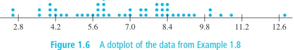
Here is data on state-by-state appropriations for higher education as a percentage of state and local tax revenue for the fiscal year 2006–2007 (from the Statistical Abstract of the United States); values are listed in order of state abbreviations (AL

first, WY last):

[image:36.576.239.469.485.544.2]

10.8 6.9 8.0 8.8 7.3 3.6 4.1 6.0 4.4 8.3 8.1 8.0 5.9 5.9 7.6 8.9 8.5 8.1 4.2 5.7 4.0 6.7 5.8 9.9 5.6 5.8 9.3 6.2 2.5 4.5 12.8 3.5 10.0 9.1 5.0 8.1 5.3 3.9 4.0 8.0 7.4 7.5 8.4 8.3 2.6 5.1 6.0 7.0 6.5 10.3

Figure 1.6 shows a dotplot of the data. The most striking feature is the substantial state-to-state variability. The largest value (for New Mexico) and the two smallest values (New Hampshire and Vermont) are somewhat separated from the bulk of the data, though not perhaps by enough to be considered outliers.

[image:36.576.242.530.628.677.2]

2.8 4.2 5.6 7.0 8.4 9.8 11.2 12.6

(37)

DEFINITION

If the number of compressive strength observations in Example 1.2 had been much larger than the actually obtained, it would be quite cumbersome to construct a dotplot. Our next technique is well suited to such situations.

Histograms

Some numerical data is obtained by counting to determine the value of a variable (the number of traffic citations a person received during the last year, the number of cus-tomers arriving for service during a particular period), whereas other data is obtained by taking measurements (weight of an individual, reaction time to a particular stimulus). The prescription for drawing a histogram is generally different for these two cases.

n527

A numerical variable is discreteif its set of possible values either is finite or else can be listed in an infinite sequence (one in which there is a first number, a second number, and so on). A numerical variable is continuousif its possi-ble values consist of an entire interval on the number line.

A discrete variable xalmost always results from counting, in which case

pos-sible values are 0, 1, 2, 3, . . . or some subset of these integers. Continuous variables arise from making measurements. For example, if xis the pH of a chemical

sub-stance, then in theory xcould be any number between 0 and 14: 7.0, 7.03, 7.032, and

so on. Of course, in practice there are limitations on the degree of accuracy of any measuring instrument, so we may not be able to determine pH, reaction time, height, and concentration to an arbitrarily large number of decimal places. However, from the point of view of creating mathematical models for distributions of data, it is help-ful to imagine an entire continuum of possible values.

Consider data consisting of observations on a discrete variable x.The frequency of any particular xvalue is the number of times that value occurs in the data set. The

relative frequencyof a value is the fraction or proportion of times the value occurs:

Suppose, for example, that our data set consists of 200 observations on

of courses a college student is taking this term. If 70 of these xvalues are 3, then

Multiplying a relative frequency by 100 gives a percentage; in the college-course example, 35% of the students in the sample are taking three courses. The relative fre-quencies, or percentages, are usually of more interest than the frequencies them-selves. In theory, the relative frequencies should sum to 1, but in practice the sum may differ slightly from 1 because of rounding. A frequency distributionis a tab-ulation of the frequencies and/or relative frequencies.

relative frequency of the x value 3: 70

200 5 .35 frequency of the x value 3: 70

x5_{the number} relative frequency of a value5 number of times the value occurs

number of observations in the data set

Constructing a Histogram for Discrete Data

First, determine the frequency and relative frequency of each xvalue. Then mark

possible xvalues on a horizontal scale. Above each value, draw a rectangle whose

(38)

Example 1.9

This construction ensures that the areaof each rectangle is proportional to the

rela-tive frequency of the value. Thus if the relarela-tive frequencies of and are .35 and .07, respectively, then the area of the rectangle above 1 is five times the area of the rectangle above 5.

How unusual is a no-hitter or a one-hitter in a major league baseball game, and how frequently does a team get more than 10, 15, or even 20 hits? Table 1.1 is a frequency distribution for the number of hits per team per game for all nine-inning games that were played between 1989 and 1993.

x5 5

[image:38.576.215.548.193.400.2]

x5 1

Table 1.1 Frequency Distribution for Hits in Nine-Inning Games

Number Relative Number of Relative

Hits/Game of Games Frequency Hits/Game Games Frequency

0 20 .0010 14 569 .0294

1 72 .0037 15 393 .0203

2 209 .0108 16 253 .0131

3 527 .0272 17 171 .0088

4 1048 .0541 18 97 .0050

5 1457 .0752 19 53 .0027

6 1988 .1026 20 31 .0016

7 2256 .1164 21 19 .0010

8 2403 .1240 22 13 .0007

9 2256 .1164 23 5 .0003

10 1967 .1015 24 1 .0001

11 1509 .0779 25 0 .0000

12 1230 .0635 26 1 .0001

13 834 .0430 27 1 .0001

19,383 1.0005

The corresponding histogram in Figure 1.7 rises rather smoothly to a single peak and then declines. The histogram extends a bit more on the right (toward large values) than it does on the left—a slight “positive skew.”

10 .05

0 .10

0 20 Hits/game

Relative frequency

[image:38.576.189.547.475.691.2]

(39)

Either from the tabulated information or from the histogram itself, we can determine the following:

Similarly,

That is, roughly 64% of all these games resulted in between 5 and 10 (inclusive)

hits. _■

Constructing a histogram for continuous data (measurements) entails subdi-viding the measurement axis into a suitable number of class intervalsor classes, such that each observation is contained in exactly one class. Suppose, for example, that we have 50 observations on efficiency of an automobile (mpg), the smallest of which is 27.8 and the largest of which is 31.4. Then we could use the class boundaries 27.5, 28.0, 28.5, . . . , and 31.5 as shown here:

x5 fuel between 5 and 10 hits (inclusive)

5 .07521 .10261c 1.10155.6361 proportion of games with

5.00101.00371 .01085 .0155 at most two hits

relative 1 _frequency

for x5 ₂ relative

1 _frequency for x5 ₁ relative

5 _frequency for x5₀ proportion of games with

27.5 28.0 28.5 29.0 29.5 30.0 30.5 31.0 31.5

One potential difficulty is that occasionally an observation lies on a class bound-ary so therefore does not fall in exactly one interval, for example, 29.0. One way to deal with this problem is to use boundaries like 27.55, 28.05, . . . , 31.55. Adding a hundredths digit to the class boundaries prevents observations from falling on the resulting boundaries. Another approach is to use the classes . Then 29.0 falls in the class rather than in the class . In other words, with this con-vention, an observation on a boundary is placed in the interval to the rightof the

boundary. This is how Minitab constructs a histogram. 28.52, 29.0 29.02, 29.5

27.52, 28.0, 28.02, 28.5, c, 31.02, 31.5

Example 1.10

Constructing a Histogram for Continuous Data: Equal Class Widths

Determine the frequency and relative frequency for each class. Mark the class boundaries on a horizontal measurement axis. Above each class inter-val, draw a rectangle whose height is the corresponding relative frequency (or frequency).

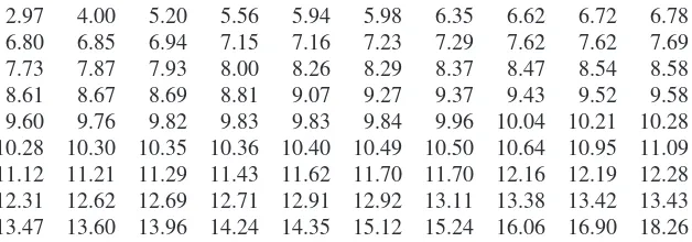
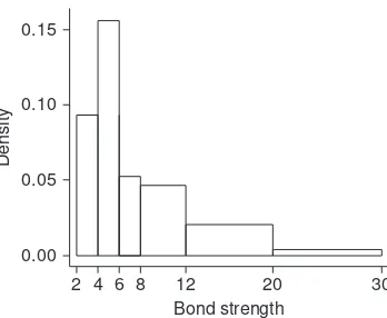
Power companies need information about customer usage to obtain accurate fore-casts of demands. Investigators from Wisconsin Power and Light determined energy consumption (BTUs) during a particular period for a sample of 90 gas-heated homes. An adjusted consumption value was calculated as follows:

This resulted in the accompanying data (part of the stored data set FURNACE.MTW available in Minitab), which we have ordered from smallest to largest.

adjusted consumption5 consumption

(40)

1 3 5 7 9 BTUIN 0

10 20 30

P

ercent

[image:40.576.226.540.52.162.2]

11 13 15 17 19

Figure 1.8 Histogram of the energy consumption data from Example 1.10 Class

Frequency 1 1 11 21 25 17 9 4 1

Relative .011 .011 .122 .233 .278 .189 .100 .044 .011 frequency

172,19 152,17

132,15 112,13

92,11 72,9

52,7 32,5 12,3

2.97 4.00 5.20 5.56 5.94 5.98 6.35 6.62 6.72 6.78

6.80 6.85 6.94 7.15 7.16 7.23 7.29 7.62 7.62 7.69

7.73 7.87 7.93 8.00 8.26 8.29 8.37 8.47 8.54 8.58

8.61 8.67 8.69 8.81 9.07 9.27 9.37 9.43 9.52 9.58

9.60 9.76 9.82 9.83 9.83 9.84 9.96 10.04 10.21 10.28 10.28 10.30 10.35 10.36 10.40 10.49 10.50 10.64 10.95 11.09 11.12 11.21 11.29 11.43 11.62 11.70 11.70 12.16 12.19 12.28 12.31 12.62 12.69 12.71 12.91 12.92 13.11 13.38 13.42 13.43 13.47 13.60 13.96 14.24 14.35 15.12 15.24 16.06 16.90 18.26

We let Minitab select the class intervals. The most striking feature of the histogram in Figure 1.8 is its resemblance to a bell-shaped (and therefore symmetric) curve, with the point of symmetry roughly at 10.

From the histogram,

The relative frequency for the class is about .27, so we estimate that roughly half of this, or .135, is between 9 and 10. Thus

The exact value of this proportion is . ■

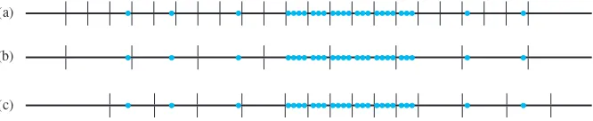
There are no hard-and-fast rules concerning either the number of classes or the choice of classes themselves. Between 5 and 20 classes will be satisfactory for most data sets. Generally, the larger the number of observations in a data set, the more classes should be used. A reasonable rule of thumb is

number of classes< 1number of observations 47/905 .522

less than 10

proportion of observations 92,11 less than 9

observations proportion of

<.371_.135 5_{.505 (slightly more than 50%)} <.011.011 .121 .235.37 (exact value5 34

(41)

(a)

(b)

[image:41.576.176.509.176.244.2]

(c)

Figure 1.9 Selecting class intervals for “varying density” data: (a) many short equal-width