Probability and Statistics for Engineers

(1)

(2)

(3)

Data from U.S. Department of Agriculture and U.S. Department of Health and Human Services. 2010. Dietary Guidelines for Americans, 2010. 6th edn. www.healthierus.gov/ dietaryguidelines .

Adequate Nutrients Within Calorie Needs

a. Consume a variety of nutrient-dense foods and beverages within and among the basic food groups while choosing foods that limit the intake of saturated and trans_fats, cholesterol, added sugars, salt, and alcohol.

b. Meet recommended intakes by adopting a balanced eating pattern, such as the USDA Food Patterns or the DASH Eating Plan.

Weight Management

a. To maintain body weight in a healthy range, balance cal-ories from foods and beverages with calcal-ories expended.

b. To prevent gradual weight gain over time, make small decreases in food and beverage calories and increase physical activity.

Physical Activity

a. Engage in regular physical activity and reduce sedentary activities to promote health, psychological well-being, and a healthy body weight.

b. Achieve physical fitness by including cardiovascular conditioning, stretching exercises for flexibility, and re-sistance exercises or calisthenics for muscle strength and endurance.

Food Groups to Encourage

a. Consume a sufficient amount of fruits and vegetables while staying within energy needs. Two cups of fruit and 2½ cups of vegetables per day are recommended for a reference 2,000-Calorie intake, with higher or lower amounts depending on the calorie level.

b. Choose a variety of fruits and vegetables each day. In particular, select from all five vegetable subgroups (dark green, orange, legumes, starchy vegetables, and other vegetables) several times a week.

c. Consume 3 or more ounce-equivalents of whole-grain products per day, with the rest of the recommended grains coming from enriched or whole-grain products.

d. Consume 3 cups per day of fat-free or low-fat milk or equivalent milk products.

Fats

a. Consume less than 10% of Calories from saturated fatty acids and less than 300 mg/day of cholesterol, and keep trans_{fatty acid consumption as low as possible.}

b. Keep total fat intake between 20% and 35% of calories, with most fats coming from sources of polyunsaturated and monounsaturated fatty acids, such as fish, nuts, and vegetable oils.

c. Choose foods that are lean, low-fat, or fat-free, and limit intake of fats and oils high in saturated and/or trans_fatty acids.

Carbohydrates

a. Choose fiber-rich fruits, vegetables, and whole grains often.

b. Choose and prepare foods and beverages with little added sugars or caloric sweeteners, such as amounts suggested by the USDA Food Patterns and the DASH Eating Plan.

c. Reduce the incidence of dental caries by practicing good oral hygiene and consuming sugar- and starch-containing foods and beverages less frequently.

Sodium and Potassium

a. Consume less than 2,300 mg of sodium (approximately 1 tsp of salt) per day.

b. Consume potassium-rich foods, such as fruits and vegetables.

Alcoholic Beverages

a. Those who choose to drink alcoholic beverages should do so sensibly and in moderation—defined as the con-sumption of up to one drink per day for women and up to two drinks per day for men.

b. Alcoholic beverages should not be consumed by some individuals, including those who cannot restrict their alcohol intake, women of childbearing age who may be-come pregnant, pregnant and lactating women, children and adolescents, individuals taking medications that can interact with alcohol, and those with specific medical conditions.

c. Alcoholic beverages should be avoided by individuals engaging in activities that require attention, skill, or coor-dination, such as driving or operating machinery.

Food Safety

a. To avoid microbial foodborne illness, clean hands, food contact surfaces, and fruits and vegetables; separate raw, cooked, and ready-to-eat foods; cook foods to a safe tem-perature; and refrigerate perishable food promptly and defrost foods properly. Meat and poultry should not be washed or rinsed.

b. Avoid unpasteurized milk and products made from unpasteurized milk or juices and raw or partially cooked eggs, meat, or poultry.

There are additional key recommendations for specific population groups. You can access all the Guidelines on the web at www.healthierus.gov/dietaryguidelines .

DIETARY GUIDELINES FOR AMERICANS, 2010

(4)

TOLERABLE UPPER INTAKE LEVELS (UL

)

Infants 0–6 mo 600 ND e _1,000 _ND _ND _ND _ND _ND

7–12 mo 600 ND 1,500 ND ND ND ND ND

Children 1–3 y 600 400 2,500 200 10 30 300 1.0 4–8 y 900 650 3,000 300 15 40 400 1.0

Males, Females

9–13 y 1,700 1,200 4,000 600 20 60 600 2.0 14–18 y 2,800 1,800 4,000 800 30 80 800 3.0 19–70 y 3,000 2,000 4,000 1,000 35 100 1,000 3.5

⬎70 y 3,000 2,000 4,000 1,000 35 100 1,000 3.5

Pregnancy

ⱕ_{18 y} 2,800 1,800 4,000 800 30 80 800 3.0 19–50 y 3,000 2,000 4,000 1,000 35 100 1,000 3.5

Lactation

ⱕ_{18 y2,800} 1,800 4,000 4,000 30 80 800 3.0 19–50 y 3,000 2,000 4,000 1,000 35 100 1,000 3.5

Life-Stage Group Vitamin A (μg/d) b

Vitamin C (mg/d) Vitamin D (IU/d) Vitamin E (mg/d)

c,d

Niacin (mg/d)

d

Vitamin B

6

(mg/d) Folate (μg/d)

d

Choline (g/d)

d

Vitamins

Infants 0–6 mo ND 1,000 ND 0.7 ND 40 ND ND ND ND ND 45 ND 4 7–12 mo ND 1,500 ND 0.9 ND 40 ND ND ND ND ND 60 ND 5

Children 1–3 y 3 2500 1,000 1.3 200 40 65 2 300 0.2 3 90 ND 7 4–8 y 6 2500 3,000 2.2 300 40 110 3 600 0.3 3 150 ND 12

Males, Females 9–13 y 11 3,000 5,000 10 600 40 350 6 1,100 0.6 4 280 ND 23 14–18 y 17 3,000 8,000 10 900 45 350 9 1,700 1.0 4 400 ND 34 19–50 y 20 2,500 10,000 10 1,100 45 350 11 2,000 1.0 4 400 1.8 40 51–70 y 2,000 70 y 20 2,000 10,000 10 1,100 45 350 11 2,000 1.0 3 400 1.8 40

Pregnancy

ⱕ18y 17 3,000 8,000 10 900 45 350 9 1,700 1.0 3.5 400 ND 34 19–50 y 20 2,500 10,000 10 1,100 45 350 11 2,000 1.0 3.5 400 ND 40

Lactation

ⱕ18y 17 3,000 8,000 10 900 45 350 9 1,700 1.0 4 400 ND 34 19–50 y 20 2,500 10,000 10 1,100 45 350 11 2,000 1.0 4 400 ND 40

Life-Stage Group Boron (mg/d)Calcium (mg/d)Copper (μg/d)Fluoride (mg/d)Iodine (μg/d)Iron (mg/d) Magnesium (mg/d)

f

Manganese (mg/d)Molybdenum (μg/d)(mg/d)Nickel (mg/d)Phosphorus (g/d)Selenium (μg/d)Vanadium (mg/d)

g

Zinc (mg/d)

Elements

From the Dietary Reference Intakes series. Copyright © 2011 by the National Academy of Sciences. Reprinted with permission by the National Academy of Sciences. Courtesy of the National Academies Press, Washington, DC.

a_UL⫽ The maximum level of daily nutrient intake that is likely to pose no risk of adverse effects. Unless otherwise specified, the UL represents total intake from food, water, and supplements. Due to lack of suitable data, ULs could not be established for vitamin K, thiamin, riboflavin, vitamin B 12 , pantothenic acid, biotin, or carotenoids. In the absence of ULs, extra caution may be warranted in consuming levels above recommended intakes.

b_{As preformed vitamin A only.}

c_As␣-tocopherol; applies to any form of supplemental ␣-tocopherol.

d_{The ULs for vitamin E, niacin, and folate apply to synthetic forms obtained from supplements, fortified foods, or a combination of the two.}

e_ND⫽ Not determinable due to lack of data of adverse effects in this age group and concern with regard to lack of ability to handle excess amounts. Source of intake should be from food only to prevent high levels of intake.

f_{The ULs for magnesium represent intake from a pharmacological agent only and do not include intake from food and water.}

g_{Although vanadium in food has not been shown to cause adverse effects in humans, there is no justification for adding vanadium to food, and vanadium supplements should be used with caution. The UL is based on adverse effects}

(5)

Essentials of Probability & Statistics

for Engineers & Scientists

Ronald E. Walpole

Roanoke College

Raymond H. Myers

Virginia Tech

Sharon L. Myers

Radford University

Keying Ye

(6)

Editor in Chief: Deirdre Lynch

Acquisitions Editor: Christopher Cummings

Executive Content Editor: Christine O’Brien

Sponsoring Editor: Christina Lepre

Associate Content Editor: Dana Bettez

Editorial Assistant: Sonia Ashraf

Senior Managing Editor: Karen Wernholm

Senior Production Project Manager: Tracy Patruno

Associate Director of Design: USHE North and West,Andrea Nix

Cover Designer: Heather Scott

Digital Assets Manager: Marianne Groth

Associate Media Producer: Jean Choe

Marketing Manager: Erin Lane

Marketing Assistant: Kathleen DeChavez

Senior Author Support/Technology Specialist: Joe Vetere

Rights and Permissions Advisor: Michael Joyce

Procurement Manager: Evelyn Beaton

Procurement Specialist: Debbie Rossi

Production Coordination: Lifland et al., Bookmakers

Composition: Keying Ye

Cover image: Marjory Dressler/Dressler Photo-Graphics

Many of the designations used by manufacturers and sellers to distinguish their products are claimed as trademarks. Where those designations appear in this book, and Pearson was aware of a trademark claim, the designations have been printed in initial caps or all caps.

Library of Congress Cataloging-in-Publication Data

Essentials of probability & statistics for engineers & scientists/Ronald E. Walpole . . . [et al.]. p. cm.

Shorter version of: Probability and statistics for engineers and scientists. c2011. ISBN 0-321-78373-5

1. Engineering—Statistical methods. 2. Probabilities. I. Walpole, Ronald E. II. Probability and statistics for engineers and scientists. III. Title: Essentials of probability and statistics for engineers and scientists.

TA340.P738 2013 620.001’5192—dc22

2011007277

Copyright c2013 Pearson Education, Inc. All rights reserved. No part of this publication may be reproduced, stored in a retrieval system, or transmitted, in any form or by any means, electronic, mechanical, photocopying, recording, or otherwise, without the prior written permission of the publisher. Printed in the United States of America. For information on obtaining permission for use of material in this work, please submit a written request to Pearson Education, Inc., Rights and Contracts Department, 501 Boylston Street, Suite 900, Boston, MA 02116, fax your request to 617-671-3447, or e-mail at http://www.pearsoned.com/legal/permissions.htm. 1 2 3 4 5 6 7 8 9 10—EB—15 14 13 12 11

www.pearsonhighered.com

(7)

2 Random Variables, Distributions,

and Expectations

. . .

49

2.1 Concept of a Random Variable . . . 49

2.2 Discrete Probability Distributions . . . 52

2.3 Continuous Probability Distributions . . . 55

Exercises . . . 59

2.4 Joint Probability Distributions . . . 62

Exercises . . . 72

2.5 Mean of a Random Variable . . . 74

(8)

2.6 Variance and Covariance of Random Variables. . . 81

Exercises . . . 88

2.7 Means and Variances of Linear Combinations of Random Variables 89 Exercises . . . 94

2.8 Potential Misconceptions and Hazards; Relationship to Material in Other Chapters . . . 99

3 Some Probability Distributions

. . .

101

3.1 Introduction and Motivation . . . 101

3.2 Binomial and Multinomial Distributions . . . 101

Exercises . . . 108

3.3 Hypergeometric Distribution . . . 109

Exercises . . . 113

3.4 Negative Binomial and Geometric Distributions . . . 114

3.5 Poisson Distribution and the Poisson Process . . . 117

Exercises . . . 120

3.6 Continuous Uniform Distribution . . . 122

3.7 Normal Distribution . . . 123

3.8 Areas under the Normal Curve . . . 126

3.9 Applications of the Normal Distribution . . . 132

Exercises . . . 135

3.10 Normal Approximation to the Binomial . . . 137

Exercises . . . 142

3.11 Gamma and Exponential Distributions . . . 143

3.12 Chi-Squared Distribution. . . 149

Exercises . . . 150

4 Sampling Distributions and Data Descriptions

157

4.1 Random Sampling . . . 157

4.2 Some Important Statistics . . . 159

Exercises . . . 162

4.3 Sampling Distributions . . . 164

4.4 Sampling Distribution of Means and the Central Limit Theorem . 165 Exercises . . . 172

(9)

Contents v

4.6 t-Distribution . . . 176

4.7 F-Distribution . . . 180

4.8 Graphical Presentation . . . 183

Exercises . . . 190

5 One- and Two-Sample Estimation Problems

195

5.1 Introduction . . . 195

5.2 Statistical Inference . . . 195

5.3 Classical Methods of Estimation. . . 196

5.4 Single Sample: Estimating the Mean . . . 199

5.5 Standard Error of a Point Estimate . . . 206

5.6 Prediction Intervals . . . 207

5.7 Tolerance Limits . . . 210

Exercises . . . 212

5.8 Two Samples: Estimating the Diﬀerence between Two Means . . . 214

5.9 Paired Observations . . . 219

Exercises . . . 221

5.10 Single Sample: Estimating a Proportion . . . 223

5.11 Two Samples: Estimating the Diﬀerence between Two Proportions 226 Exercises . . . 227

5.12 Single Sample: Estimating the Variance . . . 228

Exercises . . . 230

6 One- and Two-Sample Tests of Hypotheses

. . .

235

6.1 Statistical Hypotheses: General Concepts . . . 235

6.2 Testing a Statistical Hypothesis . . . 237

6.3 The Use of P-Values for Decision Making in Testing Hypotheses . 247 Exercises . . . 250

6.4 Single Sample: Tests Concerning a Single Mean . . . 251

6.5 Two Samples: Tests on Two Means . . . 258

6.6 Choice of Sample Size for Testing Means . . . 264

6.7 Graphical Methods for Comparing Means . . . 266

(10)

6.8 One Sample: Test on a Single Proportion. . . 272

6.9 Two Samples: Tests on Two Proportions . . . 274

Exercises . . . 276

6.10 Goodness-of-Fit Test . . . 277

6.11 Test for Independence (Categorical Data) . . . 280

6.12 Test for Homogeneity . . . 283

6.13 Two-Sample Case Study . . . 286

Exercises . . . 288

7 Linear Regression

. . .

295

7.1 Introduction to Linear Regression . . . 295

7.2 The Simple Linear Regression (SLR) Model and the Least Squares Method. . . 296

Exercises . . . 303

7.3 Inferences Concerning the Regression Coeﬃcients. . . 306

7.4 Prediction . . . 314

Exercises . . . 318

7.5 Analysis-of-Variance Approach . . . 319

7.6 Test for Linearity of Regression: Data with Repeated Observations 324 Exercises . . . 327

7.7 Diagnostic Plots of Residuals: Graphical Detection of Violation of Assumptions . . . 330

7.8 Correlation . . . 331

7.9 Simple Linear Regression Case Study. . . 333

Exercises . . . 335

7.10 Multiple Linear Regression and Estimation of the Coeﬃcients . . . 335

Exercises . . . 340

7.11 Inferences in Multiple Linear Regression . . . 343

Exercises . . . 346

8 One-Factor Experiments: General

. . .

355

8.1 Analysis-of-Variance Technique and the Strategy of Experimental Design . . . 355

(11)

Contents vii

8.3 Tests for the Equality of Several Variances . . . 364

Exercises . . . 366

8.4 Multiple Comparisons . . . 368

Exercises . . . 371

8.5 Concept of Blocks and the Randomized Complete Block Design . 372 Exercises . . . 380

8.6 Random Eﬀects Models . . . 383

8.7 Case Study for One-Way Experiment . . . 385

Exercises . . . 387

9 Factorial Experiments (Two or More Factors)

393

9.1 Introduction . . . 393

9.2 Interaction in the Two-Factor Experiment . . . 394

9.3 Two-Factor Analysis of Variance . . . 397

Exercises . . . 406

9.4 Three-Factor Experiments. . . 409

Exercises . . . 416

Bibliography

. . .

423

Appendix A: Statistical Tables and Proofs

. . .

427

Appendix B: Answers to Odd-Numbered

Non-Review Exercises

. . .

455

(12)

(13)

Preface

General Approach and Mathematical Level

This text was designed for a one-semester course that covers the essential topics needed for a fundamental understanding of basic statistics and its applications in the fields of engineering and the sciences. A balance between theory and application is maintained throughout the text. Coverage of analytical tools in statistics is enhanced with the use of calculus when discussion centers on rules and concepts in probability. Students using this text should have the equivalent of the completion of one semester of diﬀerential and integral calculus. Linear algebra would be helpful but not necessary if the instructor chooses not to include Section 7.11 on multiple linear regression using matrix algebra.

Class projects and case studies are presented throughout the text to give the student a deeper understanding of real-world usage of statistics. Class projects provide the opportunity for students to work alone or in groups to gather their own experimental data and draw inferences using the data. In some cases, the work conducted by the student involves a problem whose solution will illustrate the meaning of a concept and/or will provide an empirical understanding of an important statistical result. Case studies provide commentary to give the student a clear understanding in the context of a practical situation. The comments we aﬀectionately call “Pot Holes” at the end of each chapter present the big pic-ture and show how the chapters relate to one another. They also provide warn-ings about the possible misuse of statistical techniques presented in the chapter. A large number of exercises are available to challenge the student. These exer-cises deal with real-life scientific and engineering applications. The many data sets associated with the exercises are available for download from the website http://www.pearsonhighered.com/mathstatsresources.

Content and Course Planning

This textbook contains nine chapters. The first two chapters introduce the notion of random variables and their properties, including their role in characterizing data sets. Fundamental to this discussion is the distinction, in a practical sense, between populations and samples.

In Chapter 3, both discrete and continuous random variables are illustrated with examples. The binomial, Poisson, hypergeometric, and other useful discrete distributions are discussed. In addition, continuous distributions include the

(14)

mal, gamma, and exponential. In all cases, real-life scenarios are given to reveal how these distributions are used in practical engineering problems.

The material on specific distributions in Chapter 3 is followed in Chapter 4 by practical topics such as random sampling and the types of descriptive statistics that convey the center of location and variability of a sample. Examples involv-ing the sample mean and sample variance are included. Followinvolv-ing the introduc-tion of central tendency and variability is a substantial amount of material dealing with the importance of sampling distributions. Real-life illustrations highlight how sampling distributions are used in basic statistical inference. Central Limit type methodology is accompanied by the mechanics and purpose behind the use of the

normal, Studentt,χ2_{, and}_f _{distributions, as well as examples that illustrate their}

use. Students are exposed to methodology that will be brought out again in later chapters in the discussions of estimation and hypothesis testing. This fundamental methodology is accompanied by illustration of certain important graphical meth-ods, such as stem-and-leaf and box-and-whisker plots. Chapter 4 presents the first of several case studies involving real data.

Chapters 5 and 6 complement each other, providing a foundation for the solu-tion of practical problems in which estimasolu-tion and hypothesis testing are employed. Statistical inference involving a single mean and two means, as well as one and two proportions, is covered. Confidence intervals are displayed and thoroughly dis-cussed; prediction intervals and tolerance intervals are touched upon. Problems with paired observations are covered in detail.

In Chapter 7, the basics of simple linear regression (SLR) and multiple linear regression (MLR) are covered in a depth suitable for a one-semester course. Chap-ters 8 and 9 use a similar approach to expose students to the standard methodology associated with analysis of variance (ANOVA). Although regression and ANOVA are challenging topics, the clarity of presentation, along with case studies, class projects, examples, and exercises, allows students to gain an understanding of the essentials of both.

In the discussion of rules and concepts in probability, the coverage of analytical tools is enhanced through the use of calculus. Though the material on multiple linear regression in Chapter 7 covers the essential methodology, students are not burdened with the level of matrix algebra and relevant manipulations that they would confront in a text designed for a two-semester course.

Computer Software

Case studies, beginning in Chapter 4, feature computer printout and graphical

material generated using both SASR _{and MINITAB}R_{. The inclusion of the}

(15)

Preface xi

Supplements

Instructor’s Solutions Manual. This resource contains worked-out solutions to all

text exercises and is available for download from Pearson’s Instructor Resource Center at www.pearsonhighered.com/irc.

Student’s Solutions Manual. ISBN-10: 0-321-78399-9; ISBN-13:

978-0-321-78399-8. This resource contains complete solutions to selected exercises. It is available for purchase from MyPearsonStore at www.mypearsonstore.com, or ask your local representative for value pack options.

PowerPointR _{Lecture Slides}_{. These slides include most of the figures and tables}

from the text. Slides are available for download from Pearson’s Instructor Resource Center at www.pearsonhighered.com/irc.

Looking for more comprehensive coverage for a two-semester course? See the more

comprehensive book Probability and Statistics for Engineers and Scientists, 9th

edition, by Walpole, Myers, Myers, and Ye (ISBN-10: 0-321-62911-6; ISBN-13: 978-0-321-62911-1).

Acknowledgments

We are indebted to those colleagues who provided many helpful suggestions for this

text. They are David Groggel, Miami University; Lance Hemlow, Raritan Valley

Community College; Ying Ji,University of Texas at San Antonio; Thomas Kline,

University of Northern Iowa; Sheila Lawrence, Rutgers University; Luis Moreno,

Broome County Community College; Donald Waldman, University of Colorado—

Boulder; and Marlene Will, Spalding University. We would also like to thank

Delray Schultz, Millersville University, and Keith Friedman, University of Texas

— Austin, for ensuring the accuracy of this text.

We would like to thank the editorial and production services provided by nu-merous people from Pearson/Prentice Hall, especially the editor in chief Deirdre Lynch, acquisitions editor Chris Cummings, sponsoring editor Christina Lepre, as-sociate content editor Dana Bettez, editorial assistant Sonia Ashraf, production project manager Tracy Patruno, and copyeditor Sally Lifland. We thank the Vir-ginia Tech Statistical Consulting Center, which was the source of many real-life data sets.

(16)

Billy and Julie

R.H.M. and S.L.M.

Limin, Carolyn and Emily

(17)

Chapter 1

Introduction to Statistics

and Probability

1.1

Overview: Statistical Inference, Samples, Populations,

and the Role of Probability

Beginning in the 1980s and continuing into the 21st century, a great deal of

at-tention has been focused on improvement of qualityin American industry. Much

has been said and written about the Japanese “industrial miracle,” which began in the middle of the 20th century. The Japanese were able to succeed where we and other countries had failed—namely, to create an atmosphere that allows the production of high-quality products. Much of the success of the Japanese has

been attributed to the use of statistical methods and statistical thinking among

management personnel.

Use of Scientific Data

The use of statistical methods in manufacturing, development of food products, computer software, energy sources, pharmaceuticals, and many other areas involves

the gathering of information or scientific data. Of course, the gathering of data

is nothing new. It has been done for well over a thousand years. Data have been collected, summarized, reported, and stored for perusal. However, there is a

profound distinction between collection of scientific information and inferential

statistics. It is the latter that has received rightful attention in recent decades. The oﬀspring of inferential statistics has been a large “toolbox” of statistical methods employed by statistical practitioners. These statistical methods are de-signed to contribute to the process of making scientific judgments in the face of uncertaintyandvariation. The product density of a particular material from a manufacturing process will not always be the same. Indeed, if the process involved is a batch process rather than continuous, there will be not only variation in ma-terial density among the batches that come oﬀ the line (batch-to-batch variation), but also within-batch variation. Statistical methods are used to analyze data from a process such as this one in order to gain more sense of where in the process

changes may be made to improve thequalityof the process. In this process,

(18)

ity may well be defined in relation to closeness to a target density value in harmony

with what portion of the timethis closeness criterion is met. An engineer may be

concerned with a specific instrument that is used to measure sulfur monoxide in the air during pollution studies. If the engineer has doubts about the eﬀectiveness

of the instrument, there are two sources of variation that must be dealt with.

The first is the variation in sulfur monoxide values that are found at the same locale on the same day. The second is the variation between values observed and

thetrueamount of sulfur monoxide that is in the air at the time. If either of these

two sources of variation is exceedingly large (according to some standard set by the engineer), the instrument may need to be replaced. In a biomedical study of a new drug that reduces hypertension, 85% of patients experienced relief, while it is generally recognized that the current drug, or “old” drug, brings relief to 80% of pa-tients that have chronic hypertension. However, the new drug is more expensive to make and may result in certain side eﬀects. Should the new drug be adopted? This is a problem that is encountered (often with much more complexity) frequently by pharmaceutical firms in conjunction with the FDA (Federal Drug Administration). Again, the consideration of variation needs to be taken into account. The “85%” value is based on a certain number of patients chosen for the study. Perhaps if the study were repeated with new patients the observed number of “successes” would be 75%! It is the natural variation from study to study that must be taken into account in the decision process. Clearly this variation is important, since variation from patient to patient is endemic to the problem.

Variability in Scientific Data

In the problems discussed above the statistical methods used involve dealing with variability, and in each case the variability to be studied is that encountered in scientific data. If the observed product density in the process were always the same and were always on target, there would be no need for statistical methods. If the device for measuring sulfur monoxide always gives the same value and the value is accurate (i.e., it is correct), no statistical analysis is needed. If there were no patient-to-patient variability inherent in the response to the drug (i.e., it either always brings relief or not), life would be simple for scientists in the pharmaceutical firms and FDA and no statistician would be needed in the decision process. Statistics researchers have produced an enormous number of analytical methods that allow for analysis of data from systems like those described above. This reflects the true nature of the science that we call inferential statistics, namely, using techniques that allow us to go beyond merely reporting data to drawing conclusions (or inferences) about the scientific system. Statisticians make use of fundamental laws of probability and statistical inference to draw conclusions about

scientific systems. Information is gathered in the form of samples, or collections

of observations. The process of sampling will be introduced in this chapter, and the discussion continues throughout the entire book.

Samples are collected from populations, which are collections of all

(19)

1.1 Overview: Statistical Inference, Samples, Populations, and the Role of Probability 3

computer boards manufactured by the firm over a specific period of time. If an improvement is made in the computer board process and a second sample of boards is collected, any conclusions drawn regarding the eﬀectiveness of the change in pro-cess should extend to the entire population of computer boards produced under the “improved process.” In a drug experiment, a sample of patients is taken and each is given a specific drug to reduce blood pressure. The interest is focused on drawing conclusions about the population of those who suﬀer from hypertension.

Often, it is very important to collect scientific data in a systematic way, with planning being high on the agenda. At times the planning is, by necessity, quite limited. We often focus only on certain properties or characteristics of the items or objects in the population. Each characteristic has particular engineering or, say, biological importance to the “customer,” the scientist or engineer who seeks to learn about the population. For example, in one of the illustrations above the quality of the process had to do with the product density of the output of a process. An engineer may need to study the eﬀect of process conditions, temperature, humidity, amount of a particular ingredient, and so on. He or she can systematically move

thesefactors to whatever levels are suggested according to whatever prescription

or experimental designis desired. However, a forest scientist who is interested in a study of factors that influence wood density in a certain kind of tree cannot

necessarily design an experiment. This case may require anobservational study

in which data are collected in the field but factor levelscan not be preselected.

Both of these types of studies lend themselves to methods of statistical inference. In the former, the quality of the inferences will depend on proper planning of the experiment. In the latter, the scientist is at the mercy of what can be gathered. For example, it is sad if an agronomist is interested in studying the eﬀect of rainfall on plant yield and the data are gathered during a drought.

The importance of statistical thinking by managers and the use of statistical inference by scientific personnel is widely acknowledged. Research scientists gain much from scientific data. Data provide understanding of scientific phenomena. Product and process engineers learn a great deal in their oﬀ-line eﬀorts to improve the process. They also gain valuable insight by gathering production data (on-line monitoring) on a regular basis. This allows them to determine necessary modifications in order to keep the process at a desired level of quality.

There are times when a scientific practitioner wishes only to gain some sort of summary of a set of data represented in the sample. In other words, inferential

statistics is not required. Rather, a set of single-number statistics or descriptive

statistics is helpful. These numbers give a sense of center of the location of the data, variability in the data, and the general nature of the distribution of observations in the sample. Though no specific statistical methods leading to statistical inferenceare incorporated, much can be learned. At times, descriptive statistics are accompanied by graphics. Modern statistical software packages allow

for computation of means, medians, standard deviations, and other

(20)

The Role of Probability

From this chapter to Chapter 3, we deal with fundamental notions of probability. A thorough grounding in these concepts allows the reader to have a better under-standing of statistical inference. Without some formalism of probability theory, the student cannot appreciate the true interpretation from data analysis through modern statistical methods. It is quite natural to study probability prior to study-ing statistical inference. Elements of probability allow us to quantify the strength or “confidence” in our conclusions. In this sense, concepts in probability form a major component that supplements statistical methods and helps us gauge the strength of the statistical inference. The discipline of probability, then, provides the transition between descriptive statistics and inferential methods. Elements of probability allow the conclusion to be put into the language that the science or engineering practitioners require. An example follows that will enable the reader

to understand the notion of a P-value, which often provides the “bottom line” in

the interpretation of results from the use of statistical methods.

Example 1.1: Suppose that an engineer encounters data from a manufacturing process in which 100 items are sampled and 10 are found to be defective. It is expected and antic-ipated that occasionally there will be defective items. Obviously these 100 items represent the sample. However, it has been determined that in the long run, the company can only tolerate 5% defective in the process. Now, the elements of prob-ability allow the engineer to determine how conclusive the sample information is

regarding the nature of the process. In this case, the population conceptually

represents all possible items from the process. Suppose we learn thatif the process

is acceptable, that is, if it does produce items no more than 5% of which are

de-fective, there is a probability of 0.0282 of obtaining 10 or more defective items in a random sample of 100 items from the process. This small probability suggests that the process does, indeed, have a long-run rate of defective items that exceeds 5%. In other words, under the condition of an acceptable process, the sample in-formation obtained would rarely occur. However, it did occur! Clearly, though, it would occur with a much higher probability if the process defective rate exceeded 5% by a significant amount.

From this example it becomes clear that the elements of probability aid in the translation of sample information into something conclusive or inconclusive about the scientific system. In fact, what was learned likely is alarming information to the engineer or manager. Statistical methods, which we will actually detail in Chapter

6, produced aP-value of 0.0282. The result suggests that the processvery likely

is not acceptable. The concept of aP-valueis dealt with at length in succeeding chapters. The example that follows provides a second illustration.

(21)

1.1 Overview: Statistical Inference, Samples, Populations, and the Role of Probability 5

no nitrogen. All other environmental conditions were held constant. All seedlings

contained the fungusPisolithus tinctorus. More details are supplied in Chapter 5.

The stem weights in grams were recorded after the end of 140 days. The data are given in Table 1.1.

Table 1.1: Data Set for Example 1.2 No Nitrogen Nitrogen

0.32 0.26

0.53 0.43

0.28 0.47

0.37 0.49

0.47 0.52

0.43 0.75

0.36 0.79

0.42 0.86

0.38 0.62

0.43 0.46

0.25 0.30 0.35 0.40 0.45 0.50 0.55 0.60 0.65 0.70 0.75 0.80 0.85 0.90

Figure 1.1: A dot plot of stem weight data.

In this example there are two samples from twoseparate populations. The

purpose of the experiment is to determine if the use of nitrogen has an influence on the growth of the roots. The study is a comparative study (i.e., we seek to compare the two populations with regard to a certain important characteristic). It

is instructive to plot the data as shown in the dot plot of Figure 1.1. The◦values

represent the “nitrogen” data and the×values represent the “no-nitrogen” data.

Notice that the general appearance of the data might suggest to the reader that, on average, the use of nitrogen increases the stem weight. Four nitrogen ob-servations are considerably larger than any of the no-nitrogen obob-servations. Most of the no-nitrogen observations appear to be below the center of the data. The appearance of the data set would seem to indicate that nitrogen is eﬀective. But how can this be quantified? How can all of the apparent visual evidence be summa-rized in some sense? As in the preceding example, the fundamentals of probability can be used. The conclusions may be summarized in a probability statement or

P-value. We will not show here the statistical inference that produces the summary

probability. As in Example 1.1, these methods will be discussed in Chapter 6. The

issue revolves around the “probability that data like these could be observed”given

that nitrogen has no eﬀect, in other words, given that both samples were generated

(22)

How Do Probability and Statistical Inference Work Together?

It is important for the reader to understand the clear distinction between the discipline of probability, a science in its own right, and the discipline of inferen-tial statistics. As we have already indicated, the use or application of concepts in probability allows real-life interpretation of the results of statistical inference. As a result, it can be said that statistical inference makes use of concepts in probability. One can glean from the two examples above that the sample information is made available to the analyst and, with the aid of statistical methods and elements of probability, conclusions are drawn about some feature of the population (the pro-cess does not appear to be acceptable in Example 1.1, and nitrogen does appear to influence average stem weights in Example 1.2). Thus for a statistical problem, the sample along with inferential statistics allows us to draw conclu-sions about the population, with inferential statistics making clear use of elements of probability. This reasoning is inductivein nature. Now as we move into Section 1.4 and beyond, the reader will note that, unlike what we do in our two examples here, we will not focus on solving statistical problems. Many examples will be given in which no sample is involved. There will be a population clearly described with all features of the population known. Then questions of im-portance will focus on the nature of data that might hypothetically be drawn from

the population. Thus, one can say that elements in probability allow us to

draw conclusions about characteristics of hypothetical data taken from the population, based on known features of the population. This type of

reasoning is deductive in nature. Figure 1.2 shows the fundamental relationship

between probability and inferential statistics.

Population Sample

Probability

Statistical Inference

Figure 1.2: Fundamental relationship between probability and inferential statistics.

(23)

1.2 Sampling Procedures; Collection of Data 7

surface it would appear to be a refutation of the conjecture because 10 out of 100 seem to be “a bit much.” But without elements of probability, how do we know? Only through the study of material in future chapters will we learn the conditions under which the process is acceptable (5% defective). The probability of obtaining 10 or more defective items in a sample of 100 is 0.0282.

We have given two examples where the elements of probability provide a sum-mary that the scientist or engineer can use as evidence on which to build a decision. The bridge between the data and the conclusion is, of course, based on foundations of statistical inference, distribution theory, and sampling distributions discussed in future chapters.

1.2

Sampling Procedures; Collection of Data

In Section 1.1 we discussed very briefly the notion of sampling and the sampling process. While sampling appears to be a simple concept, the complexity of the questions that must be answered about the population or populations necessitates that the sampling process be very complex at times. While the notion of sampling is discussed in a technical way in Chapter 4, we shall endeavor here to give some common-sense notions of sampling. This is a natural transition to a discussion of the concept of variability.

Simple Random Sampling

The importance of proper sampling revolves around the degree of confidence with which the analyst is able to answer the questions being asked. Let us assume that only a single population exists in the problem. Recall that in Example 1.2 two

populations were involved. Simple random samplingimplies that any particular

sample of a specified sample size has the same chance of being selected as any

other sample of the same size. The termsample sizesimply means the number of

elements in the sample. Obviously, a table of random numbers can be utilized in sample selection in many instances. The virtue of simple random sampling is that it aids in the elimination of the problem of having the sample reflect a diﬀerent (possibly more confined) population than the one about which inferences need to be made. For example, a sample is to be chosen to answer certain questions regarding political preferences in a certain state in the United States. The sample involves the choice of, say, 1000 families, and a survey is to be conducted. Now, suppose it turns out that random sampling is not used. Rather, all or nearly all of the 1000 families chosen live in an urban setting. It is believed that political preferences in rural areas diﬀer from those in urban areas. In other words, the sample drawn actually confined the population and thus the inferences need to be confined to the “limited population,” and in this case confining may be undesirable. If, indeed, the inferences need to be made about the state as a whole, the sample of size 1000

described here is often referred to as abiased sample.

As we hinted earlier, simple random sampling is not always appropriate. Which alternative approach is used depends on the complexity of the problem. Often, for example, the sampling units are not homogeneous and naturally divide themselves

(24)

and a procedure called stratiﬁed random sampling involves random selection of a

sample within each stratum. The purpose is to be sure that each of the strata

is neither over- nor underrepresented. For example, suppose a sample survey is conducted in order to gather preliminary opinions regarding a bond referendum that is being considered in a certain city. The city is subdivided into several ethnic groups which represent natural strata. In order not to disregard or overrepresent any group, separate random samples of families could be chosen from each group.

Experimental Design

The concept of randomness or random assignment plays a huge role in the area of experimental design, which was introduced very briefly in Section 1.1 and is an important staple in almost any area of engineering or experimental science. This will also be discussed at length in Chapter 8. However, it is instructive to give a brief presentation here in the context of random sampling. A set of

so-called treatments or treatment combinationsbecomes the populations to be

studied or compared in some sense. An example is the nitrogen versus no-nitrogen treatments in Example 1.2. Another simple example would be placebo versus active drug, or in a corrosion fatigue study we might have treatment combinations that involve specimens that are coated or uncoated as well as conditions of low or high humidity to which the specimens are exposed. In fact, there are four treatment or factor combinations (i.e., 4 populations), and many scientific questions may be asked and answered through statistical and inferential methods. Consider first the situation in Example 1.2. There are 20 diseased seedlings involved in the experiment. It is easy to see from the data themselves that the seedlings are diﬀerent from each other. Within the nitrogen group (or the no-nitrogen group)

there is considerable variability in the stem weights. This variability is due to

what is generally called theexperimental unit. This is a very important concept

in inferential statistics, in fact one whose description will not end in this chapter. The nature of the variability is very important. If it is too large, stemming from a condition of excessive nonhomogeneity in experimental units, the variability will “wash out” any detectable diﬀerence between the two populations. Recall that in this case that did not occur.

The dot plot in Figure 1.1 and P-value indicated a clear distinction between

these two conditions. What role do those experimental units play in the data-taking process itself? The common-sense and, indeed, quite standard approach is

to assign the 20 seedlings or experimental units randomly to the two

treat-ments or conditions. In the drug study, we may decide to use a total of 200 available patients, patients that clearly will be diﬀerent in some sense. They are the experimental units. However, they all may have the same chronic condition

for which the drug is a potential treatment. Then in a so-calledcompletely

(25)

1.2 Sampling Procedures; Collection of Data 9

Why Assign Experimental Units Randomly?

What is the possible negative impact of not randomly assigning experimental units to the treatments or treatment combinations? This is seen most clearly in the case of the drug study. Among the characteristics of the patients that produce variability in the results are age, gender, and weight. Suppose merely by chance the placebo group contains a sample of people that are predominately heavier than those in the treatment group. Perhaps heavier individuals have a tendency to have a higher blood pressure. This clearly biases the result, and indeed, any result obtained through the application of statistical inference may have little to do with the drug and more to do with diﬀerences in weights among the two samples of patients.

We should emphasize the attachment of importance to the term variability.

Excessive variability among experimental units “camouflages” scientific findings. In future sections, we attempt to characterize and quantify measures of variability. In sections that follow, we introduce and discuss specific quantities that can be computed in samples; the quantities give a sense of the nature of the sample with respect to center of location of the data and variability in the data. A discussion of several of these single-number measures serves to provide a preview of what statistical information will be important components of the statistical methods that are used in future chapters. These measures that help characterize the nature

of the data set fall into the category ofdescriptive statistics. This material is

a prelude to a brief presentation of pictorial and graphical methods that go even further in characterization of the data set. The reader should understand that the statistical methods illustrated here will be used throughout the text. In order to oﬀer the reader a clearer picture of what is involved in experimental design studies, we oﬀer Example 1.3.

Example 1.3: A corrosion study was made in order to determine whether coating an aluminum metal with a corrosion retardation substance reduced the amount of corrosion. The coating is a protectant that is advertised to minimize fatigue damage in this type of material. Also of interest is the influence of humidity on the amount of corrosion. A corrosion measurement can be expressed in thousands of cycles to failure. Two levels of coating, no coating and chemical corrosion coating, were used. In addition, the two relative humidity levels are 20% relative humidity and 80% relative humidity.

The experiment involves four treatment combinations that are listed in the table that follows. There are eight experimental units used, and they are aluminum specimens prepared; two are assigned randomly to each of the four treatment combinations. The data are presented in Table 1.2.

The corrosion data are averages of two specimens. A plot of the averages is pictured in Figure 1.3. A relatively large value of cycles to failure represents a small amount of corrosion. As one might expect, an increase in humidity appears to make the corrosion worse. The use of the chemical corrosion coating procedure appears to reduce corrosion.

(26)

Table 1.2: Data for Example 1.3

Average Corrosion in

Coating Humidity Thousands of Cycles to Failure

Uncoated 20% 975

80% 350

Chemical Corrosion 20% 1750

80% 1550

0 1000 2000

0 20% 80%

Humidity

Average Corrosion

Uncoated Chemical Corrosion Coating

Figure 1.3: Corrosion results for Example 1.3.

conditions representing the four treatment combinations are four separate popula-tions and that the two corrosion values observed for each population are important pieces of information. The importance of the average in capturing and summariz-ing certain features in the population will be highlighted in Section 4.2. While we might draw conclusions about the role of humidity and the impact of coating the specimens from the figure, we cannot truly evaluate the results from an

analyti-cal point of view without taking into account the variability around the average.

Again, as we indicated earlier, if the two corrosion values for each treatment com-bination are close together, the picture in Figure 1.3 may be an accurate depiction. But if each corrosion value in the figure is an average of two values that are widely dispersed, then this variability may, indeed, truly “wash away” any information that appears to come through when one observes averages only. The foregoing example illustrates these concepts:

(1) random assignment of treatment combinations (coating, humidity) to experi-mental units (specimens)

(2) the use of sample averages (average corrosion values) in summarizing sample information

(27)

1.4 Probability: Sample Space and Events 11

1.3

Discrete and Continuous Data

Statistical inference through the analysis of observational studies or designed

ex-periments is used in many scientific areas. The data gathered may be discrete

or continuous, depending on the area of application. For example, a chemical engineer may be interested in conducting an experiment that will lead to condi-tions where yield is maximized. Here, of course, the yield may be in percent or grams/pound, measured on a continuum. On the other hand, a toxicologist con-ducting a combination drug experiment may encounter data that are binary in nature (i.e., the patient either responds or does not).

Great distinctions are made between discrete and continuous data in the prob-ability theory that allow us to draw statistical inferences. Often applications of

statistical inference are found when the data are count data. For example, an

en-gineer may be interested in studying the number of radioactive particles passing through a counter in, say, 1 millisecond. Personnel responsible for the eﬃciency of a port facility may be interested in the properties of the number of oil tankers arriving each day at a certain port city. In Chapter 3, several distinct scenarios, leading to diﬀerent ways of handling data, are discussed for situations with count data.

Special attention even at this early stage of the textbook should be paid to some details associated with binary data. Applications requiring statistical analysis of binary data are voluminous. Often the measure that is used in the analysis is

the sample proportion. Obviously the binary situation involves two categories.

If there are n units involved in the data and x is defined as the number that

fall into category 1, then n−x fall into category 2. Thus, x/n is the sample

proportion in category 1, and 1−x/n is the sample proportion in category 2. In

the biomedical application, 50 patients may represent the sample units, and if 20 out of 50 experienced an improvement in a stomach ailment (common to all 50)

after all were given the drug, then 20₅₀ = 0.4 is the sample proportion for which

the drug was a success and 1−0.4 = 0.6 is the sample proportion for which the

drug was not successful. Actually the basic numerical measurement for binary data is generally denoted by either 0 or 1. For example, in our medical example, a successful result is denoted by a 1 and a nonsuccess by a 0. As a result, the sample proportion is actually a sample mean of the ones and zeros. For the successful category,

x1+x2+· · ·+x50

50 =

1 + 1 + 0 +· · ·+ 0 + 1

50 =

20 50 = 0.4.

1.4

Probability: Sample Space and Events

Sample Space

In the study of statistics, we are concerned basically with the presentation and

interpretation of chance outcomes that occur in a planned study or scientific

(28)

of gas released in a chemical reaction when the concentration of an acid is varied. Hence, the statistician is often dealing with either numerical data, representing

counts or measurements, or categorical data, which can be classified according

to some criterion.

We shall refer to any recording of information, whether it be numerical or

categorical, as an observation. Thus, the numbers 2, 0, 1, and 2, representing

the number of accidents that occurred for each month from January through April during the past year at the intersection of Driftwood Lane and Royal Oak Drive,

constitute a set of observations. Similarly, the categorical data N, D, N, N, and

D, representing the items found to be defective or nondefective when five items are

inspected, are recorded as observations.

Statisticians use the wordexperimentto describe any process that generates

a set of data. A simple example of a statistical experiment is the tossing of a coin. In this experiment, there are only two possible outcomes, heads or tails. Another experiment might be the launching of a missile and observing of its velocity at specified times. The opinions of voters concerning a new sales tax can also be considered as observations of an experiment. We are particularly interested in the observations obtained by repeating the experiment several times. In most cases, the outcomes will depend on chance and, therefore, cannot be predicted with certainty. If a chemist runs an analysis several times under the same conditions, he or she will obtain diﬀerent measurements, indicating an element of chance in the experimental procedure. Even when a coin is tossed repeatedly, we cannot be certain that a given toss will result in a head. However, we know the entire set of possibilities for each toss.

Definition 1.1: _{The set of all possible outcomes of a statistical experiment is called the}_sample spaceand is represented by the symbolS.

Each outcome in a sample space is called an element or a member of the

sample space, or simply asample point. If the sample space has a finite number

of elements, we maylistthe members separated by commas and enclosed in braces.

Thus, the sample space S, of possible outcomes when a coin is flipped, may be

written

S={H, T},

whereH andTcorrespond to heads and tails, respectively.

Example 1.4: Consider the experiment of tossing a die. If we are interested in the number that shows on the top face, the sample space is

S1={1,2,3,4,5,6}.

If we are interested only in whether the number is even or odd, the sample space is simply

S2={even, odd}.

Example 1.4 illustrates the fact that more than one sample space can be used to

(29)

thanS2. If we know which element inS1 occurs, we can tell which outcome inS2

occurs; however, a knowledge of what happens inS2is of little help in determining

which element inS1occurs. In general, it is desirable to use the sample space that

gives the most information concerning the outcomes of the experiment. In some experiments, it is helpful to list the elements of the sample space systematically by

means of atree diagram.

Example 1.5: Suppose that three items are selected at random from a manufacturing process.

Each item is inspected and classified defective, D, or nondefective,N. To list the

elements of the sample space providing the most information, we construct the tree diagram of Figure 1.4. Now, the various paths along the branches of the tree give the distinct sample points. Starting with the first path, we get the sample point

DDD, indicating the possibility that all three items inspected are defective. As we

proceed along the other paths, we see that the sample space is

S={DDD, DDN, DN D, DN N, N DD, N DN, N N D, N N N}.

D

N

D

N

D

N

D DDD N DDN D DND N DNN D NDD

N NDN D NND N NNN First

Item

Second Item

Third Item

Sample Point

Figure 1.4: Tree diagram for Example 1.5.

Sample spaces with a large or infinite number of sample points are best

de-scribed by astatement or rule method. For example, if the possible outcomes

of an experiment are the set of cities in the world with a population over 1 million, our sample space is written

S={x|xis a city with a population over 1 million},

which reads “S is the set of all xsuch that x is a city with a population over 1

(30)

(x, y) on the boundary or the interior of a circle of radius 2 with center at the

origin, we write therule

S={(x, y)|x2+y2≤4}.

Whether we describe the sample space by the rule method or by listing the elements will depend on the specific problem at hand. The rule method has practi-cal advantages, particularly for many experiments where listing becomes a tedious chore.

Consider the situation of Example 1.5 in which items from a manufacturing

process are either D, defective, or N, nondefective. There are many important

statistical procedures called sampling plans that determine whether or not a “lot”

of items is considered satisfactory. One such plan involves sampling untilk

defec-tives are observed. Suppose the experiment is to sample items randomly until one defective item is observed. The sample space for this case is

S ={D, N D, N N D, N N N D, . . .}.

Events

For any given experiment, we may be interested in the occurrence of certainevents

rather than in the occurrence of a specific element in the sample space. For

in-stance, we may be interested in the eventAthat the outcome when a die is tossed is

divisible by 3. This will occur if the outcome is an element of the subsetA={3,6}

of the sample spaceS1in Example 1.4. As a further illustration, we may be

inter-ested in the event B that the number of defectives is greater than 1 in Example

1.5. This will occur if the outcome is an element of the subset

B={DDN, DN D, N DD, DDD}

of the sample spaceS.

To each event we assign a collection of sample points, which constitute a subset of the sample space. That subset represents all of the elements for which the event is true.

Definition 1.2: _An_event_{is a subset of a sample space.}

Example 1.6: Given the sample spaceS ={t | t≥0}, where t is the life in years of a certain

electronic component, then the eventAthat the component fails before the end of

the fifth year is the subsetA={t|0≤t <5}.

It is conceivable that an event may be a subset that includes the entire sample

spaceS or a subset ofS called the null set and denoted by the symbolφ, which

contains no elements at all. For instance, if we let A be the event of detecting a

microscopic organism with the naked eye in a biological experiment, then A=φ.

Also, if

B ={x|xis an even factor of 7},

thenBmust be the null set, since the only possible factors of 7 are the odd numbers

(31)

Consider an experiment where the smoking habits of the employees of a man-ufacturing firm are recorded. A possible sample space might classify an individual as a nonsmoker, a light smoker, a moderate smoker, or a heavy smoker. Let the subset of smokers be some event. Then all the nonsmokers correspond to a diﬀerent

event, also a subset ofS, which is called thecomplementof the set of smokers.

Definition 1.3: _The_complement_{of an event}_A _{with respect to} _S _{is the subset of all elements}

ofS that are not inA. We denote the complement ofAby the symbolA′_.

Example 1.7: LetRbe the event that a red card is selected from an ordinary deck of 52 playing

cards, and let S be the entire deck. Then R′ _{is the event that the card selected}

from the deck is not a red card but a black card.

Example 1.8: Consider the sample space

S={book, cell phone, mp3, paper, stationery, laptop}.

Let A = {book, stationery, laptop, paper}. Then the complement of A is A′ ₌

{cell phone, mp3}.

We now consider certain operations with events that will result in the formation of new events. These new events will be subsets of the same sample space as the

given events. Suppose thatAandBare two events associated with an experiment.

In other words,AandBare subsets of the same sample spaceS. For example, in

the tossing of a die we might letA be the event that an even number occurs and

B the event that a number greater than 3 shows. Then the subsets A={2,4,6}

andB={4,5,6} are subsets of the same sample space

S={1,2,3,4,5,6}.

Note that bothAandB will occur on a given toss if the outcome is an element of

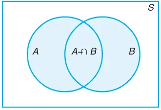
the subset{4,6}, which is just theintersection ofAandB.

Definition 1.4: _The_intersection _{of two events}_A _and_B_{, denoted by the symbol} _A_∩_B_{, is the}

event containing all elements that are common toAandB.

Example 1.9: LetE be the event that a person selected at random in a classroom is majoring

in engineering, and letF be the event that the person is female. Then E∩F is

the event of all female engineering students in the classroom.

Example 1.10: LetV ={a, e, i, o, u} andC={l, r, s, t}; then it follows thatV ∩C=φ. That is,

V andChave no elements in common and, therefore, cannot both simultaneously

occur.

For certain statistical experiments it is by no means unusual to define two

events,AandB, that cannot both occur simultaneously. The eventsAandB are

then said to bemutually exclusive. Stated more formally, we have the following

(32)

Definition 1.5: _{Two events} _A_and _B _are_{mutually exclusive}_{, or}_disjoint_{, if} _A_∩_B ₌_φ_{, that}

is, ifAandB have no elements in common.

Example 1.11: A cable television company offers programs on eight different channels, three of which are affiliated with ABC, two with NBC, and one with CBS. The other two are an educational channel and the ESPN sports channel. Suppose that a person subscribing to this service turns on a television set without first selecting

the channel. LetAbe the event that the program belongs to the NBC network and

Bthe event that it belongs to the CBS network. Since a television program cannot

belong to more than one network, the eventsAandBhave no programs in common.

Therefore, the intersection A ∩ B contains no programs, and consequently the

events AandB are mutually exclusive.

Often one is interested in the occurrence of at least one of two events associated with an experiment. Thus, in the die-tossing experiment, if

A={2,4,6}andB={4,5,6},

we might be interested in eitherAorBoccurring or bothAandBoccurring. Such

an event, called theunionofAandB, will occur if the outcome is an element of

the subset{2,4,5,6}.

Definition 1.6: _The_union_{of the two events}_A_and_B_{, denoted by the symbol}_A_∪_B_{, is the event}

containing all the elements that belong toAorB or both.

Example 1.12: LetA={a, b, c}andB={b, c, d, e}; thenA∪B={a, b, c, d, e}.

Example 1.13: Let P be the event that an employee selected at random from an oil drilling

company smokes cigarettes. LetQbe the event that the employee selected drinks

alcoholic beverages. Then the eventP ∪Q is the set of all employees who either

drink or smoke or do both.

Example 1.14: IfM ={x|3< x <9} andN={y|5< y <12}, then

M ∪N ={z|3< z <12}.

The relationship between events and the corresponding sample space can be

illustrated graphically by means of Venn diagrams. In a Venn diagram we let

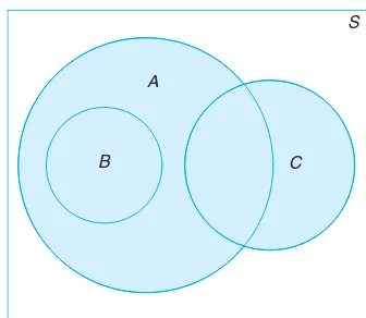
the sample space be a rectangle and represent events by circles drawn inside the rectangle. Thus, in Figure 1.5, we see that

A∩B= regions 1 and 2,

B∩C= regions 1 and 3,

A∪C= regions 1, 2, 3, 4, 5, and 7,

B′∩A= regions 4 and 7,

A∩B∩C= region 1,

(33)

A B

C

S

1

4 3

2

7 6

[image:33.540.229.397.445.591.2]

5

Figure 1.5: Events represented by various regions.

and so forth.

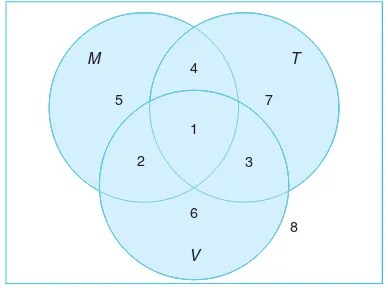
In Figure 1.6, we see that events A, B, and C are all subsets of the sample

space S. It is also clear that event B is a subset of eventA; event B∩C has no

elements and henceB andCare mutually exclusive; eventA∩C has at least one

element; and event A∪B = A. Figure 1.6 might, therefore, depict a situation

where we select a card at random from an ordinary deck of 52 playing cards and observe whether the following events occur:

A: the card is red,

B: the card is the jack, queen, or king of diamonds,

C: the card is an ace.

Clearly, the eventA∩C consists of only the two red aces.

A

B C

S

Figure 1.6: Events of the sample spaceS.

(34)

verified by means of Venn diagrams, are as follows:

1. A∩φ=φ.

2. A∪φ=A.

3. A∩A′₌_φ_.

4. A∪A′₌_S_.

5. S′₌_φ_.

6. φ′₌_S_.

7. (A′₎′₌_A_.

8. (A∩B)′ ₌_A′_∪_B′_.

9. (A∪B)′ ₌_A′_∩_B′_.

Exercises

1.1 List the elements of each of the following sample spaces:

(a) the set of integers between 1 and 50 divisible by 8; (b) the setS={x|x2_{+ 4}_x₋_{5 = 0}_}_;

(c) the set of outcomes when a coin is tossed until a tail or three heads appear;

(d) the setS={x|xis a continent}; (e) the setS={x|2x−4≥0 andx <1}.

1.2 Use the rule method to describe the sample space

S consisting of all points in the ﬁrst quadrant inside a circle of radius 3 with center at the origin.

1.3 Which of the following events are equal? (a)A={1,3};

(b)B={x|xis a number on a die}; (c)C={x|x2−4x+ 3 = 0};

(d)D={x|xis the number of heads when six coins are tossed}.

1.4 Two jurors are selected from 4 alternates to serve at a murder trial. Using the notationA1A3, for exam-ple, to denote the simple event that alternates 1 and 3 are selected, list the 6 elements of the sample spaceS.

1.5 An experiment consists of tossing a die and then ﬂipping a coin once if the number on the die is even. If the number on the die is odd, the coin is ﬂipped twice. Using the notation 4H, for example, to denote the out-come that the die out-comes up 4 and then the coin out-comes up heads, and 3HTto denote the outcome that the die comes up 3 followed by a head and then a tail on the coin, construct a tree diagram to show the 18 elements of the sample spaceS.

1.6 For the sample space of Exercise 1.5,

(a) list the elements corresponding to the eventAthat a number less than 3 occurs on the die;

(b