5
REASONS
to buy your textbooks
and course materials at
SAVINGS:
Prices up to 75% off, daily coupons, and free shipping on orders over $25
CHOICE:
Multiple format options including textbook, eBook and eChapter rentals
CONVENIENCE:
Anytime, anywhere access of eBooks or eChapters via mobile devices
SERVICE:
Free eBook access while your text ships, and instant access to online homework products
STUDY TOOLS:
Study tools
*for your text, plus writing, research, career and job search resources
*availability varies1
2
3
4
5
Find your course materials and start saving at:
www.cengagebrain.com
Engaged with you.
Australia Brazil Mexico Singapore United Kingdom United States
Probability and Statistics
for Engineering
and the Sciences
Jay Devore
ALL RIGHTS RESERVED. No part of this work covered by the copyright herein may be reproduced, transmitted, stored, or used in any form or by any means graphic, electronic, or mechanical, including but not limited to photocopying, recording, scanning, digitizing, taping, web distribution, information networks, or information storage and retrieval systems, except as permitted under Section 107 or 108 of the 1976 United States Copyright Act, without the prior written permission of the publisher.
Unless otherwise noted, all items © Cengage Learning
Library of Congress Control Number: 2014946237
ISBN: 978-1-305-25180-9
Cengage Learning
20 Channel Center Street Boston, MA 02210 USA
Cengage Learning is a leading provider of customized learning solutions with oice locations around the globe, including Singapore, the United Kingdom, Australia, Mexico, Brazil, and Japan. Locate your local oice at
www.cengage.com/global.
Cengage Learning products are represented in Canada by Nelson Education, Ltd.
To learn more about Cengage Learning Solutions, visit www.cengage.com.
Purchase any of our products at your local college store or at our preferred online store www.cengagebrain.com.
and the Sciences, Ninth Edition
Jay L. Devore
Senior Product Team Manager: Richard Stratton
Senior Product Manager: Molly Taylor
Senior Content Developer: Jay Campbell
Product Assistant: Spencer Arritt
Media Developer: Andrew Coppola
Marketing Manager: Julie Schuster
Content Project Manager: Cathy Brooks
Art Director: Linda May
Manufacturing Planner: Sandee Milewski
IP Analyst: Christina Ciaramella
IP Project Manager: Farah Fard
Production Service and Compositor: MPS Limited
Text and Cover Designer: C Miller Design
For product information and technology assistance, contact us at Cengage Learning Customer & Sales Support, 1-800-354-9706
For permission to use material from this text or product, submit all requests online at www.cengage.com/permissions
Further permissions questions can be emailed to [email protected]
Printed in the United States of America Print Number: 01 Print Year: 2014
To my beloved grandsons
Philip and Elliot, who are
vii
1
Overview and Descriptive Statistics
Introduction 1
1.1 Populations, Samples, and Processes 3
1.2 Pictorial and Tabular Methods in Descriptive Statistics 13 1.3 Measures of Location 29
1.4 Measures of Variability 36 Supplementary Exercises 47 Bibliography 51
2
Probability
Introduction 52
2.1 Sample Spaces and Events 53 2.2 Axioms, Interpretations,
and Properties of Probability 58 2.3 Counting Techniques 66 2.4 Conditional Probability 75 2.5 Independence 85
Supplementary Exercises 91 Bibliography 94
3
Discrete Random Variables and Probability
Distributions
Introduction 95 3.1 Random Variables 96
3.2 Probability Distributions for Discrete Random Variables 99 3.3 Expected Values 109
3.4 The Binomial Probability Distribution 117
3.5 Hypergeometric and Negative Binomial Distributions 126 3.6 The Poisson Probability Distribution 131
Supplementary Exercises 137 Bibliography 140
4
Continuous Random Variables and Probability
Distributions
Introduction 141
4.1 Probability Density Functions 142 4.2 Cumulative Distribution Functions
and Expected Values 147 4.3 The Normal Distribution 156
4.4 The Exponential and Gamma Distributions 170 4.5 Other Continuous Distributions 177
4.6 Probability Plots 184
Supplementary Exercises 193 Bibliography 197
5
Joint Probability Distributions
and Random Samples
Introduction 198
5.1 Jointly Distributed Random Variables 199
5.2 Expected Values, Covariance, and Correlation 213 5.3 Statistics and Their Distributions 220
5.4 The Distribution of the Sample Mean 230 5.5 The Distribution of a Linear Combination 238
Supplementary Exercises 243 Bibliography 246
6
Point Estimation
Introduction 247
6.1 Some General Concepts of Point Estimation 248 6.2 Methods of Point Estimation 264
Supplementary Exercises 274 Bibliography 275
7
Statistical Intervals Based on a Single Sample
Introduction 276
7.1 Basic Properties of Confidence Intervals 277 7.2 Large-Sample Confidence Intervals
Contents ix
7.3 Intervals Based on a Normal Population Distribution 295 7.4 Confidence Intervals for the Variance
and Standard Deviation of a Normal Population 304 Supplementary Exercises 307
Bibliography 309
8
Tests of Hypotheses Based on
a Single Sample
Introduction 310
8.1 Hypotheses and Test Procedures 311
8.2 z Tests for Hypotheses about a Population Mean 326 8.3 The One-Sample t Test 335
8.4 Tests Concerning a Population Proportion 346 8.5 Further Aspects of Hypothesis Testing 352
Supplementary Exercises 357 Bibliography 360
9
Inferences Based on Two Samples
Introduction 361
9.1 z Tests and Confidence Intervals for a Difference Between Two Population Means 362
9.2 The Two-Sample t Test and Confidence Interval 374 9.3 Analysis of Paired Data 382
9.4 Inferences Concerning a Difference Between Population Proportions 391
9.5 Inferences Concerning Two Population Variances 399 Supplementary Exercises 403
Bibliography 408
10
The Analysis of Variance
Introduction 409
10.1 Single-Factor ANOVA 410
10.2 Multiple Comparisons in ANOVA 420 10.3 More on Single-Factor ANOVA 426
11
Multifactor Analysis of Variance
Introduction 437
11.1 Two-Factor ANOVA with Kij 5 1 438 11.2 Two-Factor ANOVA with Kij . 1 451 11.3 Three-Factor ANOVA 460
11.4 2p Factorial Experiments 469
Supplementary Exercises 483 Bibliography 486
12
Simple Linear Regression and Correlation
Introduction 487
12.1 The Simple Linear Regression Model 488 12.2 Estimating Model Parameters 496
12.3 Inferences About the Slope Parameter b1 510 12.4 Inferences Concerning mY ?x* and
the Prediction of Future Y Values 519 12.5 Correlation 527
Supplementary Exercises 437 Bibliography 541
13
Nonlinear and Multiple Regression
Introduction 542
13.1 Assessing Model Adequacy 543
13.2 Regression with Transformed Variables 550 13.3 Polynomial Regression 562
13.4 Multiple Regression Analysis 572 13.5 Other Issues in Multiple Regression 595
Supplementary Exercises 610 Bibliography 618
14
Goodness-of-Fit Tests and Categorical
Data Analysis
Introduction 619
14.1 Goodness-of-Fit Tests When Category Probabilities Are Completely Specified 620
Contents xi
Supplementary Exercises 648 Bibliography 651
15
Distribution-Free Procedures
Introduction 652
15.1 The Wilcoxon Signed-Rank Test 653 15.2 The Wilcoxon Rank-Sum Test 661
15.3 Distribution-Free Confidence Intervals 667 15.4 Distribution-Free ANOVA 671
Supplementary Exercises 675 Bibliography 677
16
Quality Control Methods
Introduction 678
16.1 General Comments on Control Charts 679 16.2 Control Charts for Process Location 681 16.3 Control Charts for Process Variation 690 16.4 Control Charts for Attributes 695 16.5 CUSUM Procedures 700
16.6 Acceptance Sampling 708 Supplementary Exercises 714 Bibliography 715
Appendix Tables
A.1 Cumulative Binomial Probabilities A-2 A.2 Cumulative Poisson Probabilities A-4 A.3 Standard Normal Curve Areas A-6 A.4 The Incomplete Gamma Function A-8 A.5 Critical Values for t Distributions A-9
A.6 Tolerance Critical Values for Normal Population Distributions A-10 A.7 Critical Values for Chi-Squared Distributions A-11
A.8 t Curve Tail Areas A-12
A.9 Critical Values for F Distributions A-14
A.10 Critical Values for Studentized Range Distributions A-20 A.11 Chi-Squared Curve Tail Areas A-21
A.12 Approximate Critical Values for the Ryan-Joiner Test of Normality A-23
A.14 Critical Values for the Wilcoxon Rank-Sum Test A-25 A.15 Critical Values for the Wilcoxon Signed-Rank Interval A-26 A.16 Critical Values for the Wilcoxon Rank-Sum Interval A-27 A.17 b Curves for t Tests A-28
Answers to Selected Odd-Numbered Exercises A-29 Glossary of Symbols /Abbreviations G-1
xiii
Purpose
The use of probability models and statistical methods for analyzing data has become common practice in virtually all scientific disciplines. This book attempts to provide a comprehensive introduction to those models and methods most likely to be encoun-tered and used by students in their careers in engineering and the natural sciences. Although the examples and exercises have been designed with scientists and engi-neers in mind, most of the methods covered are basic to statistical analyses in many other disciplines, so that students of business and the social sciences will also profit from reading the book.
Approach
Students in a statistics course designed to serve other majors may be initially skeptical of the value and relevance of the subject matter, but my experience is that students can be turned on to statistics by the use of good examples and exercises that blend their everyday experiences with their scientific interests. Consequently, I have worked hard to find examples of real, rather than artificial, data—data that someone thought was worth collecting and analyzing. Many of the methods presented, especially in the later chapters on statistical inference, are illustrated by analyzing data taken from published sources, and many of the exercises also involve working with such data. Sometimes the reader may be unfamiliar with the context of a particular problem (as indeed I often was), but I have found that students are more attracted by real problems with a somewhat strange context than by patently artificial problems in a familiar setting.
Mathematical Level
The exposition is relatively modest in terms of mathematical development. Substantial use of the calculus is made only in Chapter 4 and parts of Chapters 5 and 6. In par-ticular, with the exception of an occasional remark or aside, calculus appears in the inference part of the book only—in the second section of Chapter 6. Matrix algebra is not used at all. Thus almost all the exposition should be accessible to those whose mathematical background includes one semester or two quarters of differential and integral calculus.
Content
Chapter 1 begins with some basic concepts and terminology—population, sample, descriptive and inferential statistics, enumerative versus analytic studies, and so on— and continues with a survey of important graphical and numerical descriptive methods. A rather traditional development of probability is given in Chapter 2, followed by prob-ability distributions of discrete and continuous random variables in Chapters 3 and 4, respectively. Joint distributions and their properties are discussed in the first part of Chapter 5. The latter part of this chapter introduces statistics and their sampling distri-butions, which form the bridge between probability and inference. The next three
chapters cover point estimation, statistical intervals, and hypothesis testing based on a single sample. Methods of inference involving two independent samples and paired data are presented in Chapter 9. The analysis of variance is the subject of Chapters 10 and 11 (single-factor and multifactor, respectively). Regression makes its initial appearance in Chapter 12 (the simple linear regression model and correlation) and returns for an extensive encore in Chapter 13. The last three chapters develop chi-squared methods, distribution-free (nonparametric) procedures, and techniques from statistical quality control.
Helping Students Learn
Although the book’s mathematical level should give most science and engineering students little difficulty, working toward an understanding of the concepts and gaining an appreciation for the logical development of the methodology may sometimes require substantial effort. To help students gain such an understanding and appreci-ation, I have provided numerous exercises ranging in difficulty from many that involve routine application of text material to some that ask the reader to extend concepts discussed in the text to somewhat new situations. There are many more exercises than most instructors would want to assign during any particular course, but I recommend that students be required to work a substantial number of them. In a problem-solving discipline, active involvement of this sort is the surest way to identify and close the gaps in understanding that inevitably arise. Answers to most odd-numbered exercises appear in the answer section at the back of the text. In addition, a Student Solutions Manual, consisting of worked-out solutions to virtu-ally all the odd-numbered exercises, is available.
To access additional course materials and companion resources, please visit www.cengagebrain.com. At the CengageBrain.com home page, search for the ISBN of your title (from the back cover of your book) using the search box at the top of the page. This will take you to the product page where free companion resources can be found.
New for This Edition
The major change for this edition is the elimination of the rejection region approach to hypothesis testing. Conclusions from a hypothesis-testing analysis are now based entirely on P-values. This has necessitated completely rewriting Section 8.1, which now introduces hypotheses and then test procedures based on P-values. Substantial revision of the remaining sections of Chapter 8 was then required, and this in turn has been propagated through the hypothesis-testing sections and subsections of Chapters 9–15.
Many new examples and exercises, almost all based on real data or actual problems. Some of these scenarios are less technical or broader in scope than what has been included in previous editions—for example, investigating the nocebo effect (the inclination of those told about a drug’s side effects to experi-ence them), comparing sodium contents of cereals produced by three different manufacturers, predicting patient height from an easy-to-measure anatomical characteristic, modeling the relationship between an adolescent mother’s age and the birth weight of her baby, assessing the effect of smokers’ short-term abstinence on the accurate perception of elapsed time, and exploring the impact of phrasing in a quantitative literacy test.
Preface xv
The exposition has been polished whenever possible to help students gain a better intuitive understanding of various concepts.
Acknowledgments
My colleagues at Cal Poly have provided me with invaluable support and feedback over the years. I am also grateful to the many users of previous editions who have made suggestions for improvement (and on occasion identified errors). A special note of thanks goes to Jimmy Doi for his accuracy checking and to Matt Carlton for his work on the two solutions manuals, one for instructors and the other for students.
Xianggui Qu, Oakland University; Kingsley Reeves, University of South Florida; Steve Rein, California Polytechnic State University–San Luis Obispo; Tony Richardson, University of Evansville; Don Ridgeway, North Carolina State University; Larry J. Ringer, Texas A & M University; Nabin Sapkota, University of Central Florida; Robert M. Schumacher, Cedarville University; Ron Schwartz, Florida Atlantic University; Kevan Shafizadeh, California State University– Sacramento; Mohammed Shayib, Prairie View A&M; Alice E. Smith, Auburn University; James MacGregor Smith, University of Massachusetts; Paul J. Smith, University of Maryland; Richard M. Soland, The George Washington University; Clifford Spiegelman, Texas A & M University; Jery Stedinger, Cornell University; David Steinberg, Tel Aviv University; William Thistleton, State University of New York Institute of Technology; J A Stephen Viggiano, Rochester Institute of Technology; G. Geoffrey Vining, University of Florida; Bhutan Wadhwa, Cleveland State University; Gary Wasserman, Wayne State University; Elaine Wenderholm, State University of New York–Oswego; Samuel P. Wilcock, Messiah College; Michael G. Zabetakis, University of Pittsburgh; and Maria Zack, Point Loma Nazarene University.
Preeti Longia Sinha of MPS Limited has done a terrific job of supervis-ing the book’s production. Once again I am compelled to express my grat itude to all those people at Cengage who have made important contributions over the course of my textbook writing career. For this most recent edition, special thanks go to Jay Campbell (for his timely and informed feedback throughout the project), Molly Taylor, Ryan Ahern, Spencer Arritt, Cathy Brooks, and Andrew Coppola. I also greatly appreciate the stellar work of all those Cengage Learning sales representatives who have labored to make my books more visible to the statistical community. Last but by no means least, a heartfelt thanks to my wife Carol for her decades of support, and to my daughters for providing inspiration through their own achievements.
1
Overview and
Descriptive Statistics
1
I N T R O D U C T I O N
Statistical concepts and methods are not only useful but indeed often indis-pensable in understanding the world around us. They provide ways of gaining new insights into the behavior of many phenomena that you will encounter in your chosen field of specialization in engineering or science.
The discipline of statistics teaches us how to make intelligent judgments and informed decisions in the presence of uncertainty and variation. Without uncertainty or variation, there would be little need for statistical methods or stat-isticians. If every component of a particular type had exactly the same lifetime, if all resistors produced by a certain manufacturer had the same resistance value,
“I took statistics at business school, and it was a transformative experience. Analytical training gives you a skill set that differen-tiates you from most people in the labor market.”
—LASZLO BOCK, SENIOR VICE PRESIDENTOF PEOPLE OPERATIONS (INCHARGEOFALLHIRING) AT
April 20, 2014, The New York Times, interview with columnist Thomas Friedman
“I am not much given to regret, so I puzzled over this one a while. Should have taken much more statistics in college, I think.”
—MAX LEVCHIN, PAYPAL CO-FOUNDER, SLIDE FOUNDER
Quote of the week from the Web site of the American Statistical Association on November 23, 2010
“I keep saying that the sexy job in the next 10 years will be statisti-cians, and I’m not kidding.”
—HAL VARIAN, CHIEF ECONOMISTAT GOOGLE
if pH determinations for soil specimens from a particular locale gave identical results, and so on, then a single observation would reveal all desired information.
An interesting manifestation of variation appeared in connection with determining the “greenest” way to travel. The article “CarbonConundrum” (Consumer Reports, 2008: 9) identified organizations that help consumers calculate carbon output. The following results on output for a flight from New York to Los Angeles were reported:
Carbon Calculator CO2 (lb)
Terra Pass 1924
Conservation International 3000
Cool It 3049
World Resources Institute/Safe Climate 3163 National Wildlife Federation 3465 Sustainable Travel International 3577
Native Energy 3960
Environmental Defense 4000 Carbonfund.org 4820 The Climate Trust/CarbonCounter.org 5860 Bonneville Environmental Foundation 6732
There is clearly rather substantial disagreement among these calculators as to exactly how much carbon is emitted, characterized in the article as “from a ballerina’s to Bigfoot’s.” A website address was provided where readers could learn more about how the various calculators work.
How can statistical techniques be used to gather information and draw conclusions? Suppose, for example, that a materials engineer has developed a coating for retarding corrosion in metal pipe under specified circumstances. If this coating is applied to different segments of pipe, variation in environmental conditions and in the segments themselves will result in more substantial corro-sion on some segments than on others. Methods of statistical analysis could be used on data from such an experiment to decide whether the average amount of corrosion exceeds an upper specification limit of some sort or to predict how much corrosion will occur on a single piece of pipe.
1.1 Populations, Samples, and Processes 3
between the two coatings attributable not to the coatings themselves, but just to extraneous variation. Statistics offers not only methods for analyzing the results of experiments once they have been carried out but also suggestions for how experi-ments can be performed in an efficient manner to mitigate the effects of variation and have a better chance of producing correct conclusions.
Engineers and scientists are constantly exposed to collections of facts, or data, both in their professional capacities and in everyday activities. The discipline of statistics provides methods for organizing and summarizing data and for drawing conclusions based on information contained in the data.
An investigation will typically focus on a well-defined collection of objects constituting a population of interest. In one study, the population might consist of all gelatin capsules of a particular type produced during a specified period. Another investigation might involve the population consisting of all individuals who received a B.S. in engineering during the most recent academic year. When desired informa-tion is available for all objects in the populainforma-tion, we have what is called a census. Constraints on time, money, and other scarce resources usually make a census impractical or infeasible. Instead, a subset of the population—a sample—is selected in some prescribed manner. Thus we might obtain a sample of bearings from a par-ticular production run as a basis for investigating whether bearings are conforming to manufacturing specifications, or we might select a sample of last year’s engineering graduates to obtain feedback about the quality of the engineering curricula.
We are usually interested only in certain characteristics of the objects in a pop-ulation: the number of flaws on the surface of each casing, the thickness of each capsule wall, the gender of an engineering graduate, the age at which the individual graduated, and so on. A characteristic may be categorical, such as gender or type of malfunction, or it may be numerical in nature. In the former case, the value of the characteristic is a category (e.g., female or insufficient solder), whereas in the latter case, the value is a number (e.g., age523 years or diameter5.502 cm). A variable is any characteristic whose value may change from one object to another in the population. We shall initially denote variables by lowercase letters from the end of our alphabet. Examples include
x5brand of calculator owned by a student
y5number of visits to a particular Web site during a specified period z5braking distance of an automobile under specified conditions
Data results from making observations either on a single variable or simultaneously on two or more variables. A univariate data set consists of observations on a single variable. For example, we might determine the type of transmission, automatic (A) or manual (M), on each of ten automobiles recently purchased at a certain dealer-ship, resulting in the categorical data set
M A A A M A A M A A
The following sample of pulse rates (beats per minute) for patients recently admitted to an adult intensive care unit is a numerical univariate data set:
We have bivariate data when observations are made on each of two variables. Our data set might consist of a (height, weight) pair for each basketball player on a team, with the first observation as (72, 168), the second as (75, 212), and so on. If an engineer determines the value of both x5component lifetime and y5reason for component failure, the resulting data set is bivariate with one variable numeri-cal and the other categorical. Multivariate data arises when observations are made on more than one variable (so bivariate is a special case of multivariate). For exam-ple, a research physician might determine the systolic blood pressure, diastolic blood pressure, and serum cholesterol level for each patient participating in a study. Each observation would be a triple of numbers, such as (120, 80, 146). In many multivariate data sets, some variables are numerical and others are categorical. Thus the annual automobile issue of Consumer Reports gives values of such variables as type of vehicle (small, sporty, compact, mid-size, large), city fuel efficiency (mpg), highway fuel efficiency (mpg), drivetrain type (rear wheel, front wheel, four wheel), and so on.
Branches of Statistics
An investigator who has collected data may wish simply to summarize and describe important features of the data. This entails using methods from descriptive statistics. Some of these methods are graphical in nature; the construction of histograms, boxplots, and scatter plots are primary examples. Other descriptive methods involve calculation of numerical summary measures, such as means, standard deviations, and correlation coef-ficients. The wide availability of statistical computer software packages has made these tasks much easier to carry out than they used to be. Computers are much more efficient than human beings at calculation and the creation of pictures (once they have received appropriate instructions from the user!). This means that the investigator doesn’t have to expend much effort on “grunt work” and will have more time to study the data and extract important messages. Throughout this book, we will present output from various packages such as Minitab, SAS, JMP, and R. The R software can be downloaded without charge from the site http://www.r-project.org. It has achieved great popularity in the statistical community, and many books describing its various uses are available (it does entail programming as opposed to the pull-down menus of Minitab and JMP).
Charity is a big business in the United States. The Web site charitynavigator.com gives information on roughly 6000 charitable organizations, and there are many smaller charities that fly below the navigator’s radar screen. Some charities operate very efficiently, with fundraising and administrative expenses that are only a small percentage of total expenses, whereas others spend a high percentage of what they take in on such activities. Here is data on fundraising expenses as a percentage of total expenditures for a random sample of 60 charities:
6.1 12.6 34.7 1.6 18.8 2.2 3.0 2.2 5.6 3.8 2.2 3.1 1.3 1.1 14.1 4.0 21.0 6.1 1.3 20.4 7.5 3.9 10.1 8.1 19.5 5.2 12.0 15.8 10.4 5.2 6.4 10.8 83.1 3.6 6.2 6.3 16.3 12.7 1.3 0.8 8.8 5.1 3.7 26.3 6.0 48.0 8.2 11.7 7.2 3.9 15.3 16.6 8.8 12.0 4.7 14.7 6.4 17.0 2.5 16.2
Without any organization, it is difficult to get a sense of the data’s most prominent features—what a typical (i.e., representative) value might be, whether values are highly concentrated about a typical value or quite dispersed, whether there are any gaps in the data, what fraction of the values are less than 20%, and so on. Figure 1.1
1.1 Populations, Samples, and Processes 5
shows what is called a stem-and-leaf display as well as a histogram. In Section 1.2 we will discuss construction and interpretation of these data summaries. For the moment, we hope you see how they begin to describe how the percentages are dis-tributed over the range of possible values from 0 to 100. Clearly a substantial major-ity of the charities in the sample spend less than 20% on fundraising, and only a few percentages might be viewed as beyond the bounds of sensible practice. ■
Having obtained a sample from a population, an investigator would frequently like to use sample information to draw some type of conclusion (make an inference of some sort) about the population. That is, the sample is a means to an end rather than an end in itself. Techniques for generalizing from a sample to a population are gathered within the branch of our discipline called inferential statistics.
Material strength investigations provide a rich area of application for statistical meth ods. The article “Effects of Aggregates and Microfillers on the Flexural Properties of Concrete” (Magazine of Concrete Research, 1997: 81–98) reported on a study of strength properties of high-performance concrete obtained by using superplasticizers and certain binders. The compressive strength of such concrete had previously been investigated, but not much was known about flexural strength (a measure of ability to resist failure in bending). The accompanying data on flexural strength (in MegaPascal, MPa, where 1 Pa (Pascal)51.4531024 psi) appeared in the article
cited:
5.9 7.2 7.3 6.3 8.1 6.8 7.0 7.6 6.8 6.5 7.0 6.3 7.9 9.0
8.2 8.7 7.8 9.7 7.4 7.7 9.7 7.8 7.7 11.6 11.3 11.8 10.7
Suppose we want an estimate of the average value of flexural strength for all beams that could be made in this way (if we conceptualize a population of all such beams, we are trying to estimate the population mean). It can be shown that, with a high degree of confidence, the population mean strength is between 7.48 MPa and 8.80 MPa; we call this a confidence interval or interval estimate. Alternatively, this data could be used to predict the flexural strength of a single beam of this type. With a high degree of confidence, the strength of a single such beam will exceed 7.35 MPa; the number 7.35 is called a lower prediction bound. ■ ExamplE 1.2
0 0 10 20
Fr
equency
30 40 Stem–and–leaf of FundRsng N = 60 Leaf Unit = 1.0
0 0111112222333333344 0 55556666666778888 1 0001222244 1 55666789 2 01
2 6
3 3 4
4 8
5 5 6 6 7 7
8 3
4
10 20 30 40 50 FundRsng
60 70 80 90
Figure 1.1 A Minitab stem-and-leaf display (tenths digit truncated) and histogram for the charity
The main focus of this book is on presenting and illustrating methods of inferential statistics that are useful in scientific work. The most important types of inferential procedures—point estimation, hypothesis testing, and estimation by confidence intervals—are introduced in Chapters 6–8 and then used in more com-plicated settings in Chapters 9–16. The remainder of this chapter presents methods from descriptive statistics that are most used in the development of inference.
Chapters 2–5 present material from the discipline of probability. This mate-rial ultimately forms a bridge between the descriptive and inferential techniques. Mastery of probability leads to a better understanding of how inferential procedures are developed and used, how statistical conclusions can be translated into everyday language and interpreted, and when and where pitfalls can occur in applying the methods. Probability and statistics both deal with questions involving populations and samples, but do so in an “inverse manner” to one another.
In a probability problem, properties of the population under study are assumed known (e.g., in a numerical population, some specified distribution of the population values may be assumed), and questions regarding a sample taken from the population are posed and answered. In a statistics problem, characteristics of a sample are available to the experimenter, and this information enables the experi-menter to draw conclusions about the population. The relationship between the two disciplines can be summarized by saying that probability reasons from the popu-lation to the sample (deductive reasoning), whereas inferential statistics rea sons from the sample to the population (inductive reasoning). This is illustrated in Figure 1.2.
Population
Probability
Inferential statistics
Sample
Figure 1.2 The relationship between probability and inferential statistics
Before we can understand what a particular sample can tell us about the popu-lation, we should first understand the uncertainty associated with taking a sample from a given population. This is why we study probability before statistics.
As an example of the contrasting focus of probability and inferential statistics, con-sider drivers’ use of manual lap belts in cars equipped with automatic shoulder belt systems. (The article “Automobile Seat Belts: Usage Patterns in Automatic Belt Systems,” Human Factors,1998: 126–135, summarizes usage data.) In probability, we might assume that 50% of all drivers of cars equipped in this way in a certain metropolitan area regularly use their lap belt (an assumption about the population), so we might ask, “How likely is it that a sample of 100 such drivers will include at least 70 who regularly use their lap belt?” or “How many of the drivers in a sample of size 100 can we expect to regularly use their lap belt?” On the other hand, in infer-ential statistics, we have sample information available; for example, a sample of 100 drivers of such cars revealed that 65 regularly use their lap belt. We might then ask, “Does this provide substantial evidence for concluding that more than 50% of all such drivers in this area regularly use their lap belt?” In this latter scenario, we are attempting to use sample information to answer a question about the structure of the entire population from which the sample was selected. ■
In the foregoing lap belt example, the population is well defined and concrete: all drivers of cars equipped in a certain way in a particular metropolitan area. In Example 1.2, however, the strength measurements came from a sample of prototype beams that
1.1 Populations, Samples, and Processes 7
had not been selected from an existing population. Instead, it is conven ient to think of the population as consisting of all possible strength measurements that might be made under similar experimental conditions. Such a population is referred to as a conceptual or hypothetical population. There are a number of prob lem situations in which we fit questions into the framework of inferential statistics by conceptualizing a population.
The Scope of Modern Statistics
These days statistical methodology is employed by investigators in virtually all dis-ciplines, including such areas as
● molecular biology (analysis of microarray data)
● ecology (describing quantitatively how individuals in various animal and plant
populations are spatially distributed)
● materials engineering (studying properties of various treatments to retard corrosion)
● marketing (developing market surveys and strategies for marketing new products)
● public health (identifying sources of diseases and ways to treat them)
● civil engineering (assessing the effects of stress on structural elements and the
impacts of traffic flows on communities)
As you progress through the book, you’ll encounter a wide spectrum of different sce-narios in the examples and exercises that illustrate the application of techniques from probability and statistics. Many of these scenarios involve data or other material extracted from articles in engineering and science journals. The methods presented herein have become established and trusted tools in the arsenal of those who work with data. Meanwhile, statisticians continue to develop new models for describing rand-omness, and uncertainty and new methodology for analyzing data. As evidence of the continuing creative efforts in the statistical community, here are titles and capsule descriptions of some articles that have recently appeared in statistics journals (Journal of the American Statistical Association is abbreviated JASA, and AAS is short for the Annals of Applied Statistics, two of the many prominent journals in the discipline):
● “How Many People Do You Know? Efficiently Estimating Personal
Network Size” (JASA, 2010: 59–70): How many of the N individuals at your college do you know? You could select a random sample of students from the population and use an estimate based on the fraction of people in this sam-ple that you know. Unfortunately this is very inefficient for large populations because the fraction of the population someone knows is typically very small. A “latent mixing model” was proposed that the authors asserted remedied deficien-cies in previously used techniques. A simulation study of the method’s effec-tiveness based on groups consisting of first names (“How many people named Michael do you know?”) was included as well as an application of the method to actual survey data. The article concluded with some practical guidelines for the construction of future surveys designed to estimate social network size.
● “Active Learning Through Sequential Design, with Applications to the
● “Robust Internal Benchmarking and False Discovery Rates for Detecting
Racial Bias in Police Stops”(JASA, 2009: 661–668): Allegations of police actions that are attributable at least in part to racial bias have become a contentious issue in many communities. This article proposes a new method that is designed to reduce the risk of flagging a substantial number of “false positives” (individuals falsely identified as manifesting bias). The method was applied to data on 500,000 pedestrian stops in New York City in 2006; of the 3000 officers regu larly involved in pedestrian stops, 15 were identified as having stopped a sub stantially greater frac-tion of Black and Hispanic people than what would be predicted were bias absent.
● “Records in Athletics Through Extreme Value Theory” (JASA, 2008:
1382–1391):The focus here is on the modeling of extremes related to world records in athletics. The authors start by posing two questions: (1) What is the ultimate world record within a specific event (e.g., the high jump for women)? and (2) How “good” is the current world record, and how does the quality of current world records compare across different events? A total of 28 events (8 running, 3 throwing, and 3 jumping for both men and women) are consid-ered. For example, one conclusion is that only about 20 seconds can be shaved off the men’s marathon record, but that the current women’s marathon record is almost 5 minutes longer than what can ultimately be achieved. The method-ology also has applications to such issues as ensuring airport runways are long enough and that dikes in Holland are high enough.
● “Self-Exciting Hurdle Models for Terrorist Activity”(AAS, 2012: 106–124): The
authors developed a predictive model of terrorist activity by considering the daily number of terrorist attacks in Indonesia from 1994 through 2007. The model esti-mates the chance of future attacks as a function of the times since past attacks. One feature of the model considers the excess of nonattack days coupled with the pres-ence of multiple coordinated attacks on the same day. The article provides an inter-pretation of various model characteristics and assesses its predictive performance.
● “Prediction of Remaining Life of Power Transformers Based on Left
Truncated and Right Censored Lifetime Data” (AAS, 2009: 857–879): There are roughly 150,000 high-voltage power transmission transformers in the United States. Unexpected failures can cause substantial economic losses, so it is impor-tant to have predictions for remaining lifetimes. Relevant data can be complicated because lifetimes of some transformers extend over several decades during which records were not necessarily complete. In particular, the authors of the article use data from a certain energy company that began keeping careful records in 1980. But some transformers had been installed before January 1, 1980, and were still in service after that date (“left truncated” data), whereas other units were still in service at the time of the investigation, so their complete lifetimes are not available (“right censored” data). The article describes various procedures for obtaining an interval of plausible values (a prediction interval) for a remaining lifetime and for the cumulative number of failures over a specified time period.
● “The BARISTA: A Model for Bid Arrivals in Online Auctions” (AAS,2007:
1.1 Populations, Samples, and Processes 9
then validated using data from eBay.com on auctions for Palm M515 personal assistants, Microsoft Xbox games, and Cartier watches.
● “Statistical Challenges in the Analysis of Cosmic Microwave Background
Radiation” (AAS, 2009: 61–95):The cosmic microwave background (CMB) is a significant source of information about the early history of the universe. Its radiation level is uniform, so extremely delicate instruments have been developed to measure fluctuations. The authors provide a review of statistical issues with CMB data analysis; they also give many examples of the application of statistical procedures to data obtained from a recent NASA satellite mission, the Wilkinson Microwave Anisotropy Probe.
Statistical information now appears with increasing frequency in the popular media, and occasionally the spotlight is even turned on statisticians. For example, the Nov. 23, 2009,New York Times reported in an article “Behind Cancer Guidelines, Quest for Data” that the new science for cancer investigations and more sophisticated methods for data analysis spurred the U.S. Preventive Services task force to re-examine guide-lines for how frequently middle-aged and older women should have mammograms. The panel commissioned six independent groups to do statistical modeling. The result was a new set of conclusions, including an assertion that mammograms every two years are nearly as beneficial to patients as annual mammograms, but confer only half the risk of harms. Donald Berry, a very prominent biostatistician, was quoted as saying he was pleasantly surprised that the task force took the new research to heart in making its recommendations. The task force’s report has generated much controversy among cancer organizations, politicians, and women themselves.
It is our hope that you will become increasingly convinced of the importance and relevance of the discipline of statistics as you dig more deeply into the book and the subject. Hopefully you’ll be turned on enough to want to continue your statistical education beyond your current course.
Enumerative Versus Analytic Studies
W. E. Deming, a very influential American statistician who was a moving force in Japan’s quality revolution during the 1950s and 1960s, introduced the distinction between enumerative studies and analytic studies. In the former, interest is focused on a finite, identifiable, unchanging collection of individuals or objects that make up a population. A sampling frame—that is, a listing of the individuals or objects to be sampled—is either available to an investigator or else can be constructed. For exam-ple, the frame might consist of all signatures on a petition to qualify a certain initia-tive for the ballot in an upcoming election; a sample is usually selected to ascertain whether the number of valid signatures exceeds a specified value. As another example, the frame may contain serial numbers of all furnaces manufactured by a particular company during a certain time period; a sample may be selected to infer something about the average lifetime of these units. The use of inferential methods to be developed in this book is reasonably noncontroversial in such settings (though statisticians may still argue over which particular methods should be used).
tested to investigate efficiency. These five could be viewed as a sample from the concep-tual population of all prototypes that could be manufactured under similar conditions, but not necessarily as representative of the population of units manufactured once regular production gets underway. Methods for using sample information to draw conclusions about future production units may be problematic. Someone with expertise in the area of turbine design and engineering (or whatever other subject area is relevant) should be called upon to judge whether such extrapolation is sensible. A good exposition of these issues is contained in the article “Assumptions for Statistical Inference” by Gerald Hahn and William Meeker (The American Statistician, 1993: 1–11).
Collecting Data
Statistics deals not only with the organization and analysis of data once it has been collected but also with the development of techniques for collecting the data. If data is not properly collected, an investigator may not be able to answer the questions under consideration with a reasonable degree of confidence. One common problem is that the target population—the one about which conclusions are to be drawn—may be different from the population actually sampled. For example, advertisers would like various kinds of information about the television-viewing habits of potential cus-tomers. The most systematic information of this sort comes from placing monitoring devices in a small number of homes across the United States. It has been conjectured that placement of such devices in and of itself alters viewing behavior, so that charac-teristics of the sample may be different from those of the target population.
When data collection entails selecting individuals or objects from a frame, the simplest method for ensuring a representative selection is to take a simple random sample. This is one for which any particular subset of the specified size (e.g., a sam-ple of size 100) has the same chance of being selected. For examsam-ple, if the frame consists of 1,000,000 serial numbers, the numbers 1, 2, … , up to 1,000,000 could be placed on identical slips of paper. After placing these slips in a box and thor-oughly mixing, slips could be drawn one by one until the requisite sample size has been obtained. Alternatively (and much to be preferred), a table of random numbers or a software package’s random number generator could be employed.
Sometimes alternative sampling methods can be used to make the selection process easier, to obtain extra information, or to increase the degree of confidence in conclusions. One such method, stratified sampling, entails separating the population units into nonoverlapping groups and taking a sample from each one. For example, a study of how physicians feel about the Affordable Care Act might proceed by stratifying according to specialty: select a sample of surgeons, another sample of radiologists, yet another sample of psychiatrists, and so on. This would result in information separately from each specialty and ensure that no one specialty is over- or underrepresented in the entire sample.
Frequently a “convenience” sample is obtained by selecting individuals or objects without systematic randomization. As an example, a collection of bricks may be stacked in such a way that it is extremely difficult for those in the center to be selected. If the bricks on the top and sides of the stack were somehow different from the others, resulting sample data would not be representative of the population. Often an investigator will assume that such a convenience sample approximates a random sample, in which case a statistician’s repertoire of inferential methods can be used; however, this is a judgment call. Most of the methods discussed herein are based on a variation of simple random sampling described in Chapter 5.
1.1 Populations, Samples, and Processes 11
of land or pieces of pipe). Alternatively, an investigator may systematically vary the levels or categories of certain factors (e.g., pressure or type of insulating material) and observe the effect on some response variable (such as yield from a production process).
An article in the New York Times(Jan. 27, 1987) reported that heart attack risk could be reduced by taking aspirin. This conclusion was based on a designed experi ment involv-ing both a control group of individuals that took a placebo havment involv-ing the appearance of aspirin but known to be inert and a treatment group that took aspirin according to a specified regimen. Subjects were randomly assigned to the groups to protect against any biases and so that probability-based methods could be used to analyze the data. Of the 11,034 individuals in the control group, 189 subsequently experienced heart attacks, whereas only 104 of the 11,037 in the aspirin group had a heart attack. The incidence rate of heart attacks in the treatment group was only about half that in the control group. One possible explanation for this result is chance variation—that aspirin really doesn’t have the desired effect and the observed difference is just typical variation in the same way that tossing two identical coins would usually produce different numbers of heads. However, in this case, inferential methods suggest that chance variation by itself cannot adequately explain the magnitude of the observed difference. ■
An engineer wishes to investigate the effects of both adhesive type and conductor material on bond strength when mounting an integrated circuit (IC) on a certain sub-strate. Two adhesive types and two conductor materials are under consideration. Two observations are made for each adhesive-type/conductor-material combination, resulting in the accompanying data:
ExamplE 1.4
ExamplE 1.5
Adhesive Type Conductor Material Observed Bond Strength Average
1 1 82, 77 79.5
1 2 75, 87 81.0
2 1 84, 80 82.0
2 2 78, 90 84.0
The resulting average bond strengths are pictured in Figure 1.3. It appears that adhe-sive type 2 improves bond strength as compared with type 1 by about the same amount whichever one of the conducting materials is used, with the 2, 2 combin-ation being best. Inferential methods can again be used to judge whether these effects are real or simply due to chance variation.
Conducting material Average
strength
1 2
80 85
Adhesive type 2
Adhesive type 1
Figure 1.3 Average bond strengths in Example 1.5
factors, and our engineer may not have enough resources to make even a single observa-tion for each of these combinaobserva-tions. In Chapter 11, we will see how the careful selecobserva-tion of a fraction of these possibilities will usually yield the desired information. ■
1. Give one possible sample of size 4 from each of the fol-lowing populations:
a. All daily newspapers published in the United States b. All companies listed on the New York Stock
Exchange
c. All students at your college or university
d. All grade point averages of students at your college or university
2. For each of the following hypothetical populations, give a plausible sample of size 4:
a. All distances that might result when you throw a football
b. Page lengths of books published 5 years from now c. All possible earthquake-strength measurements
(Richter scale) that might be recorded in California during the next year
d. All possible yields (in grams) from a certain chemi-cal reaction carried out in a laboratory
3. Consider the population consisting of all computers of a certain brand and model, and focus on whether a com-puter needs service while under warranty.
a. Pose several probability questions based on selecting a sample of 100 such computers.
b. What inferential statistics question might be answered by determining the number of such computers in a sample of size 100 that need warranty service?
4. a. Give three different examples of concrete popula-tions and three different examples of hypothetical populations.
b. For one each of your concrete and your hypothetical populations, give an example of a probability question and an example of an inferential statistics question.
5. Many universities and colleges have instituted supplemen-tal instruction (SI) programs, in which a student facilitator meets regularly with a small group of students enrolled in the course to promote discussion of course material and enhance subject mastery. Suppose that students in a large statistics course (what else?) are randomly divided into a control group that will not participate in SI and a treatment group that will participate. At the end of the term, each student’s total score in the course is determined.
a. Are the scores from the SI group a sample from an existing population? If so, what is it? If not, what is the relevant conceptual population?
b. What do you think is the advantage of randomly dividing the students into the two groups rather than letting each student choose which group to join? c. Why didn’t the investigators put all students in the
treat-ment group? [Note: The article “Supplemental Instruction: An Effective Component of Student Affairs Programming” (J. of College Student Devel., 1997: 577–586) discusses the analysis of data from several SI programs.]
6. The California State University (CSU) system consists of 23 campuses, from San Diego State in the south to Humboldt State near the Oregon border. A CSU admin-istrator wishes to make an inference about the average distance between the hometowns of students and their campuses. Describe and discuss several different sam-pling methods that might be employed. Would this be an enumerative or an analytic study? Explain your reasoning.
7. A certain city divides naturally into ten district neighbor-hoods. How might a real estate appraiser select a sample of single-family homes that could be used as a basis for developing an equation to predict appraised value from characteristics such as age, size, number of bathrooms, distance to the nearest school, and so on? Is the study enumerative or analytic?
8. The amount of flow through a solenoid valve in an auto-mobile’s pollution-control system is an important char-acteristic. An experiment was carried out to study how flow rate depended on three factors: armature length, spring load, and bobbin depth. Two different levels (low and high) of each factor were chosen, and a single observation on flow was made for each combination of levels.
a. The resulting data set consisted of how many observations?
b. Is this an enumerative or analytic study? Explain your reasoning.
1.2 Pictorial and Tabular Methods in Descriptive Statistics 13
1.2
Pictorial and Tabular Methods
in Descriptive Statistics
Descriptive statistics can be divided into two general subject areas. In this section, we consider representing a data set using visual displays. In Sections 1.3 and 1.4, we will develop some numerical summary measures for data sets. Many visual techniques may already be familiar to you: frequency tables, tally sheets, histograms, pie charts, bar graphs, scatter diagrams, and the like. Here we focus on a selected few of these techniques that are most useful and relevant to probability and inferential statistics.
Notation
Some general notation will make it easier to apply our methods and formulas to a wide variety of practical problems. The number of observations in a single sample, that is, the sample size, will often be denoted by n, so that n54 for the sample of universities {Stanford, Iowa State, Wyoming, Rochester} and also for the sample of pH measurements {6.3, 6.2, 5.9, 6.5}. If two samples are simultaneously under con-sideration, either m and n or n1 and n2 can be used to denote the numbers of
observa-tions. An experiment to compare thermal efficiencies for two different types of diesel engines might result in samples {29.7, 31.6, 30.9} and {28.7, 29.5, 29.4, 30.3}, in which case m53 and n54.
Given a data set consisting of n observations on some variable x, the individ-ual observations will be denoted by x1, x2, x3,…, xn. The subscript bears no relation to the magnitude of a particular observation. Thus x1 will not in general be the
small-est observation in the set, nor will xn typically be the largest. In many applications, x1 will be the first observation gathered by the experimenter, x2 the second, and so
on. The ith observation in the data set will be denoted by xi.
Stem-and-Leaf Displays
Consider a numerical data set x1, x2,…, xn for which each xi consists of at least two digits. A quick way to obtain an informative visual representation of the data set is to construct a stem-and-leaf display.
Constructing a Stem-and-Leaf Display
1. Select one or more leading digits for the stem values. The trailing digits become the leaves.
2. List possible stem values in a vertical column.
3. Record the leaf for each observation beside the corresponding stem value. 4. Indicate the units for stems and leaves someplace in the display.
with only three rows. In this case, it is desirable to stretch the display by repeating each stem value twice—9H, 9L, 8H, . . . ,7L—once for high leaves 9, . . . , 5 and again for low leaves 4, . . . , 0. Then a score of 93 would have a stem of 9L and leaf of 3. In general, a display based on between 5 and 20 stems is recommended.
A common complaint among college students is that they are getting less sleep than they need. The article “Class Start Times, Sleep, and Academic Performance in College: A Path Analysis” (Chronobiology Intl., 2012: 318–335)investigated fac-tors that impact sleep time. The stem-and-leaf display in Figure 1.4 shows the average number of hours of sleep per day over a two-week period for a sample of 253 students.
ExamplE 1.6
Figure 1.4 Stem-and-leaf display for average sleep time per day
5L 5H
00 6889
000111123444444 55556778899999
Stem: ones digit Leaf: tenths digit
000011111112222223333333344444444
55555555666666666666777777888888888999999999999999
00000000000011111122222222222222222333333333334444444444444
6L 6H 7L 7H 8L
5555555566666666677777788888888899999999999 00001111111222223334
666678999 00
56
8H 9L 9H 10L 10H
The first observation in the top row of the display is 5.0, corresponding to a stem of 5 and leaf of 0, and the last observation at the bottom of the display is 10.6. Note that in the absence of a context, without the identification of stem and leaf digits in the display, we wouldn’t know whether the observation with stem 7 and leaf 9 was .79, 7.9, or 79. The leaves in each row are ordered from smallest to larg-est; this is commonly done by software packages but is not necessary if a display is created by hand.
The display suggests that a typical or representative sleep time is in the stem 8L row, perhaps 8.1 or 8.2. The data is not highly concentrated about this typical value as would be the case if almost all students were getting between 7.5 and 9.5 hours of sleep on average. The display appears to rise rather smoothly to a peak in the 8L row and then decline smoothly (we conjecture that the minor peak in the 6L row would disappear if more data was available). The general shape of the display is rather symmetric, bearing strong resemblance to a bell-shaped curve; it does not stretch out more in one direction than the other. The two smallest and two largest values seem a bit separated from the remainder of the data—perhaps they are very mild, but certainly not extreme,“outliers”. A reference in the cited article suggests that individuals in this age group need about 8.4 hours of sleep per day. So it appears that a substantial percentage of students in the sample are sleep deprived. ■
A stem-and-leaf display conveys information about the following aspects of the data:
● identification of a typical or representative value
● extent of spread about the typical value
1.2 Pictorial and Tabular Methods in Descriptive Statistics 15
● extent of symmetry in the distribution of values
● number and locations of peaks
● presence of any outliers—values far from the rest of the data
Figure 1.5 presents stem-and-leaf displays for a random sample of lengths of golf courses (yards) that have been designated by Golf Magazine as among the most chal-lenging in the United States. Among the sample of 40 courses, the shortest is 6433 yards long, and the longest is 7280 yards. The lengths appear to be distributed in a roughly uniform fashion over the range of values in the sample. Notice that a stem choice here of either a single digit (6 or 7) or three digits (643, … , 728) would yield an uninformative display, the first because of too few stems and the latter because of too many.
ExamplE 1.7
64 35 64 33 70 Stem: Thousands and hundreds digits
65 26 27 06 83 Leaf: Tens and ones digits
66 05 94 14
67 90 70 00 98 70 45 13 68 90 70 73 50
69 00 27 36 04
70 51 05 11 40 50 22 71 31 69 68 05 13 65 72 80 09
Stem-and-leaf of yardage N 40
Leaf Unit 10
4 64 3367
8 65 0228
11 66 019
18 67 0147799
(4) 68 5779
18 69 0023
14 70 012455
8 71 013666
2 72 08
(a) (b)
Figure 1.5 Stem-and-leaf displays of golf course lengths: (a) two-digit leaves; (b) display from
Minitab with truncated one-digit leaves
Statistical software packages do not generally produce displays with multiple-digit stems. The Minitab display in Figure 1.5(b) results from truncating each obser-vation by deleting the ones digit. ■
Dotplots
A dotplot is an attractive summary of numerical data when the data set is reasonably small or there are relatively few distinct data values. Each observation is represented by a dot above the corresponding location on a horizontal measurement scale. When a value occurs more than once, there is a dot for each occurrence, and these dots are stacked vertically. As with a stem-and-leaf display, a dotplot gives information about location, spread, extremes, and gaps.
There is growing concern in the U.S. that not enough students are graduating from college. America used to be number 1 in the world for the percentage of adults with college degrees, but it has recently dropped to 16th. Here is data on the percentage of 25- to 34-year-olds in each state who had some type of postsecond-ary degree as of 2010 (listed in alphabetical order, with the District of Columbia included):
31.5 32.9 33.0 28.6 37.9 43.3 45.9 37.2 68.8 36.2 35.5 40.5 37.2 45.3 36.1 45.5 42.3 33.3 30.3 37.2 45.5 54.3 37.2 49.8 32.1 39.3 40.3 44.2 28.4 46.0 47.2 28.7 49.6 37.6 50.8 38.0 30.8 37.6 43.9 42.5 35.2 42.2 32.8 32.2 38.5 44.5 44.6 40.9 29.5 41.3 35.4
Figure 1.6 shows a dotplot of the data. Dots corresponding to some values close together (e.g., 28.6 and 28.7) have been vertically stacked to prevent crowding. There is clearly a great deal of state-to-state variability. The largest value, for D.C., is obviously an extreme outlier, and four other values on the upper end of the data are candidates for mild outliers (MA, MN, NY, and ND). There is also a cluster of states at the low end, primarily located in the South and Southwest. The overall percentage for the entire country is 39.3%; this is not a simple average of the 51 numbers but an average weighted by population sizes.
25 30 35 40 45 50 55 60 65 70
Figure 1.6 A dotplot of the data from Example 1.8 n
A dotplot can be quite cumbersome to construct and look crowded when the number of observations is large. Our next technique is well suited to such situations.
Histograms
Some numerical data is obtained by counting to determine the value of a variable (the number of traffic citations a person received during the last year, the number of custom-ers arriving for service during a particular period), whereas other data is obtained by taking measurements (weight of an individual, reaction time to a particular stimulus). The prescription for drawing a histogram is generally different for these two cases.
A numerical variable is discrete if its set of possible values either is finite or else can be listed in an infinite sequence (one in which there is a first number, a second number, and so on). A numerical variable is continuous if its possible values consist of an entire interval on the number line.
DEFINITION
A discrete variable x almost always results from counting, in which case pos-sible values are 0, 1, 2, 3, … or some subset of these integers. Continuous variables arise from making measurements. For example, if x is the pH of a chemical sub-stance, then in theory x could be any number between 0 and 14: 7.0, 7.03, 7.032, and so on. Of course, in practice there are limitations on the degree of accuracy of any measuring instrument, so we may not be able to determine pH, reaction time, height, and concentration to an arbitrarily large number of decimal places. However, from the point of view of creating mathematical models for distributions of data, it is help-ful to imagine an entire continuum of possible values.
Consider data consisting of observations on a discrete variable x. The frequency of any particular x value is the number of times that value occurs in the data set. The relative frequency of a value is the fraction or proportion of times the value occurs:
relative frequency of a value5 number of times the value occurs number of observations in the data set
Suppose, for example, that our data set consists of 200 observations on x5the number of courses a college student is taking this term. If 70 of these x values are 3, then
frequency of the x value 3:
70
1.2 Pictorial and Tabular Methods in Descriptive Statistics 17
Multiplying a relative frequency by 100 gives a percentage; in the college-course example, 35% of the students in the sample are taking three courses. The relative fre quencies, or percentages, are usually of more interest than the frequencies them-selves. In theory, the relative frequencies should sum to 1, but in practice the sum may differ slightly from 1 because of rounding. A frequency distribution is a tabu-lation of the frequencies and/or relative frequencies.
Constructing a Histogram for Discrete Data
First, determine the frequency and relative frequency of each x value. Then mark possible x values on a horizontal scale. Above each value, draw a rectangle whose height is the relative frequency (or alternatively, the frequency) of that value; the rectangles should have equal widths.
This construction ensures that the area of each rectangle is proportional to the rela-tive frequency of the value. Thus if the relarela-tive frequencies of x51 and x55 are .35 and .07, respectively, then the area of the rectangle above 1 is five times the area of the rectangle above 5.
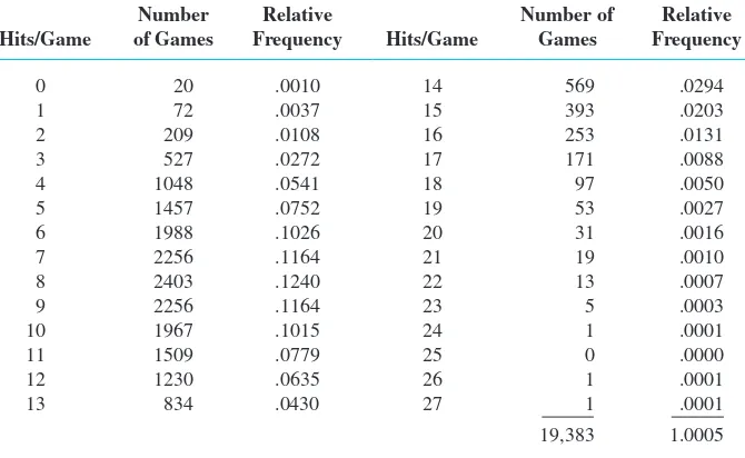
How unusual is a no-hitter or a one-hitter in a major league baseball game, and how frequently does a team get more than 10, 15, or even 20 hits? Table 1.1 is a frequency distribution for the number of hits per team per game for all nine-inning games that were played between 1989 and 1993.
ExamplE 1.9
Table 1.1 Frequency Distribution for Hits in Nine-Inning Games
Number Relative Number of Relative Hits/Game of Games Frequency Hits/Game Games Frequency
0 20 .0010 14 569 .0294
1 72 .0037 15 393 .0203
2 209 .0108 16 253 .0131
3 527 .0272 17 171 .0088
4 1048 .0541 18 97 .0050
5 1457 .0752 19 53 .0027
6 1988 .1026 20 31 .0016
7 2256 .1164 21 19 .0010
8 2403 .1240 22 13 .0007
9 2256 .1164 23 5 .0003
10 1967 .1015 24 1 .0001
11 1509 .0779 25 0 .0000
12 1230 .0635 26 1 .0001
13 834 .0430 27 1 .0001
19,383 1.0005
Either from the tabulated information or from the histogram itself, we can determine the following:
proportion of games with at most two hits
5
relative frequency
for x50 1
relative frequency
for x51 1
relative frequency
for x52 5.00101.00371.01085.0155
Similarly,
proportion of games with between 5 and 10 hits (inclusive)
5.07521.10261…1.10155.6361
That is, roughly 64% of all these games resulted in between 5 and 10 (inclusive)
hits. ■
Constructing a histogram for continuous data (measurements) entails subdividing the measurement axis into a suitable number of class intervals or classes, such that each observation is contained in exactly one class. Suppose, for example, that we have 50 observations on x5fuel efficiency of an automobile (mpg), the smallest of which is 27.8 and the largest of which is 31.4. Then we could use the class bounda-ries 27.5, 28.0, 28.5, … , and 31.5 as shown here:
10 .05
0 .10
0
Hits/game 20
Relative frequency
Figure 1.7 Histogram of number of hits per nine-inning game
27.5 28.0 28.5 29.0 29.5 30.0 30.5 31.0 31.5
1.2 Pictorial and Tabular Methods in Descriptive Statistics 19
Power companies need information about customer usage to obtain accurate fore-casts of demands. Investigators from Wisconsin Power and Light determined energy consumption (BTUs) during a particular period for a sample of 90 gas-heated homes. An adjusted consumption value was calculated as follows:
adjusted consumption5 consumption
(weather, in degree days)(house area)
This resulted in the accompanying data (part of the stored data set FURNACE.MTW available in Minitab), which we have ordered from smal