FUNDAMENTALS OF PROBABILITY AND STATISTICS FOR ENGINEERS

(1)

(2)

AND STATISTICS FOR ENGINEERS

T.T. Soong

(3)

(4)

(5)

(6)

AND STATISTICS FOR ENGINEERS

T.T. Soong

(7)

Telephone ( 44) 1243 779777

Email (for orders and customer service enquiries): cs-books@wiley.co.uk Visit our H ome Page on www.wileyeurope.com or www.wiley.com

All R ights R eserved. N o part of this publication may be reproduced, stored in a retrieval system or transmitted in any form or by any means, electronic, mechanical, photocopying, recording, scanning or otherwise, except under the terms of the Copyright, D esigns and Patents Act 1988 or under the terms of a licence issued by the Copyright Licensing Agency Ltd, 90 Tottenham Court R oad, London W1T 4LP, U K , without the permission in writing of the Publisher. R equests to the Publisher should be addressed to the Permissions D epartment, John Wiley & Sons Ltd, The Atrium, Southern G ate, Chichester, West Sussex PO19 8SQ, England, or emailed to permreq@wiley.co.uk, or faxed to ( 44) 1243 770620.

This publication is designed to provide accurate and authoritative information in regard to the subject matter covered. It is sold on the understanding that the Publisher is not engaged in rendering professional services. If professional advice or other expert assistance is required, the services of a competent professional should be sought.

Other W iley Editorial Offices

John Wiley & Sons Inc., 111 R iver Street, H oboken, N J 07030, U SA Jossey-Bass, 989 M arket Street, San F rancisco, CA 94103-1741, U SA Wiley-VCH Verlag G mbH , Boschstr. 12, D -69469 Weinheim, G ermany

John Wiley & Sons Australia Ltd, 33 Park R oad, M ilton, Queensland 4064, Australia John Wiley & Sons (Asia) Pte Ltd, 2 Clementi Loop #02-01, Jin Xing D istripark, Singapore 129809

John Wiley & Sons Canada Ltd, 22 Worcester Road, Etobicoke, Ontario, Canada M9W 1L1 Wiley also publishes its books in a variety of electronic formats. Some content that appears in print may not be available in electronic books.

British Library Cataloguing in Publication Data

A catalogue record for this book is available from the British Library ISBN 0-470-86813-9 (Cloth)

ISBN 0-470-86814-7 (Paper)

Typeset in 10/12pt Times from LaTeX files supplied by the author, processed by Integra Software Services, Pvt. Ltd, Pondicherry, India

Printed and bound in G reat Britain by Biddles Ltd, G uildford, Surrey

(8)

(9)

(10)

Preface

This book was written for an introductory one-semester or two-quarter course in probability and statistics for students in engineering and applied sciences. N o previous knowledge of probability or statistics is presumed but a good under-standing of calculus is a prerequisite for the material.

The development of this book was guided by a number of considerations observed over many years of teaching courses in this subject area, including the following:

.

_{As an introductory course, a sound and rigorous treatment of the basic} principles is imperative for a proper understanding of the subject matter and for confidence in applying these principles to practical problem solving. A student, depending upon his or her major field of study, will no doubt pursue advanced work in this area in one or more of the many possible directions. H ow well is he or she prepared to do this strongly depends on his or her mastery of the fundamentals.

.

_{It is important that the student develop an early appreciation for} tions. D emonstrations of the utility of this material in nonsuperficial applica-tions not only sustain student interest but also provide the student with stimulation to delve more deeply into the fundamentals.

.

_{M ost of the students in engineering and applied sciences can only devote one} semester or two quarters to a course of this nature in their programs. R ecognizing that the coverage is time limited, it is important that the material be self-contained, representing a reasonably complete and applicable body of knowledge.

(17)

Practical examples are emphasized; they are purposely selected from many different fields and not slanted toward any particular applied area. The same objective is observed in making up the exercises at the back of each chapter.

Because of the self-imposed criterion of writing a comprehensive text and presenting it within a limited time frame, there is a tight continuity from one topic to the next. Some flexibility exists in Chapters 6 and 7 that include discussions on more specialized distributions used in practice. F or example, extreme-value distributions may be bypassed, if it is deemed necessary, without serious loss of continuity. Also, Chapter 11 on linear models may be deferred to a follow-up course if time does not allow its full coverage.

It is a pleasure to acknowledge the substantial help I received from students in my courses over many years and from my colleagues and friends. Their constructive comments on preliminary versions of this book led to many improvements. M y sincere thanks go to M rs. Carmella G osden, who efficiently typed several drafts of this book. As in all my undertakings, my wife, D ottie, cared about this project and gave me her loving support for which I am deeply grateful.

(18)

1 Introduction

At present, almost all undergraduate curricula in engineering and applied sciences contain at least one basic course in probability and statistical inference. The recognition of this need for introducing the ideas of probability theory in a wide variety of scientific fields today reflects in part some of the profound changes in science and engineering education over the past 25 years.

One of the most significant is the greater emphasis that has been placed upon complexity and precision. A scientist now recognizes the importance of study-ing scientific phenomena havstudy-ing complex interrelations among their compon-ents; these components are often not only mechanical or electrical parts but also ‘soft-science’ in nature, such as those stemming from behavioral and social sciences. The design of a comprehensive transportation system, for example, requires a good understanding of technological aspects of the problem as well as of the behavior patterns of the user, land-use regulations, environmental requirements, pricing policies, and so on.

Moreover, precision is stressed – precision in describing interrelationships among factors involved in a scientific phenomenon and precision in predicting its behavior. This, coupled with increasing complexity in the problems we face, leads to the recognition that a great deal of uncertainty and variability are inevitably present in problem formulation, and one of the mathematical tools that is effective in dealing with them is probability and statistics.

Probabilistic ideas are used in a wide variety of scientific investigations involving randomness. Randomness is an empirical phenomenon characterized by the property that the quantities in which we are interested do not have a predictable outcome under a given set of circumstances, but instead there is a statistical regularity associated with different possible outcomes. Loosely speaking, statistical regularity means that, in observing outcomes of an

exper-iment a large number of times (sayn), the ratiom/n, wheremis the number of

observed occurrences of a specific outcome, tends to a unique limit as n

becomes large. For example, the outcome of flipping a coin is not predictable

but there is statistical regularity in that the ratiom/n approaches1

(19)

heads or tails. Random phenomena in scientific areas abound: noise in radio signals, intensity of wind gusts, mechanical vibration due to atmospheric dis-turbances, Brownian motion of particles in a liquid, number of telephone calls made by a given population, length of queues at a ticket counter, choice of transportation modes by a group of individuals, and countless others. It is not inaccurate to say that randomness is present in any realistic conceptual model of a real-world phenomenon.

1.1 ORGANIZATION OF TEXT

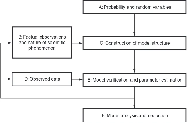
This book is concerned with the development of basic principles in constructing probability models and the subsequent analysis of these models. As in other scientific modeling procedures, the basic cycle of this undertaking consists of a number of fundamental steps; these are schematically presented in Figure 1.1. A basic understanding of probability theory and random variables is central to the whole modeling process as they provide the required mathematical machin-ery with which the modeling process is carried out and consequences deduced. The step from B to C in Figure 1.1 is the induction step by which the structure of the model is formed from factual observations of the scientific phenomenon under study. Model verification and parameter estimation (E) on the basis of observed data (D) fall within the framework of statistical inference. A model

B:Factual observations and nature of scientific

phenomenon

D:Observed data

F:Model analysis and deduction E:Model verification and parameter estimation

C:Construction of model structure A:Probability and random variables

(20)

may be rejected at this stage as a result of inadequate inductive reasoning or insufficient or deficient data. A reexamination of factual observations or add-itional data may be required here. Finally, model analysis and deduction are made to yield desired answers upon model substantiation.

In line with this outline of the basic steps, the book is divided into two parts. Part A (Chapters 2–7) addresses probability fundamentals involved in steps

A!C, B!C, and E!F (Figure 1.1). Chapters 2–5 provide these

funda-mentals, which constitute the foundation of all subsequent development. Some important probability distributions are introduced in Chapters 6 and 7. The nature and applications of these distributions are discussed. An understanding of the situations in which these distributions arise enables us to choose an appropriate distribution, or model, for a scientific phenomenon.

Part B (Chapters 8–11) is concerned principally with step D!E (Figure 1.1),

the statistical inference portion of the text. Starting with data and data repre-sentation in Chapter 8, parameter estimation techniques are carefully developed in Chapter 9, followed by a detailed discussion in Chapter 10 of a number of selected statistical tests that are useful for the purpose of model verification. In Chapter 11, the tools developed in Chapters 9 and 10 for parameter estimation and model verification are applied to the study of linear regression models, a very useful class of models encountered in science and engineering.

The topics covered in Part B are somewhat selective, but much of the foundation in statistical inference is laid. This foundation should help the reader to pursue further studies in related and more advanced areas.

1.2 PROBABILITY TABLES AND COMPUTER SOFTWARE

The application of the materials in this book to practical problems will require calculations of various probabilities and statistical functions, which can be time consuming. To facilitate these calculations, some of the probability tables are provided in Appendix A. It should be pointed out, however, that a large number of computer software packages and spreadsheets are now available that provide this information as well as perform a host of other statistical

calculations. As an example, some statistical functions available in MicrosoftÕ

ExcelTM2000 are listed in Appendix B.

1.3 PREREQUISITES

(21)

(22)

Part A

(23)

(24)

2 Basic Probability Concepts

The mathematical theory of probability gives us the basic tools for constructing and analyzing mathematical models for random phenomena. In studying a random phenomenon, we are dealing with an experiment of which the outcome is not predictable in advance. Experiments of this type that immediately come to mind are those arising in games of chance. In fact, the earliest development of probability theory in the fifteenth and sixteenth centuries was motivated by problems of this type (for example, see Todhunter, 1949).

In science and engineering, random phenomena describe a wide variety of situations. By and large, they can be grouped into two broad classes. The first class deals with physical or natural phenomena involving uncertainties. U ncer-tainty enters into problem formulation through complexity, through our lack of understanding of all the causes and effects, and through lack of information. Consider, for example, weather prediction. Information obtained from satellite tracking and other meteorological information simply is not sufficient to permit a reliable prediction of what weather condition will prevail in days ahead. It is therefore easily understandable that weather reports on radio and television are made in probabilistic terms.

The second class of problems widely studied by means of probabilistic models concerns those exhibiting variability. Consider, for example, a problem in traffic flow where an engineer wishes to know the number of vehicles cross-ing a certain point on a road within a specified interval of time. This number varies unpredictably from one interval to another, and this variability reflects variable driver behavior and is inherent in the problem. This property forces us to adopt a probabilistic point of view, and probability theory provides a powerful tool for analyzing problems of this type.

(25)

2.1 ELEMENTS OF SET THEORY

Our interest in the study of a random phenomenon is in the statements we can make concerning the events that can occur. Events and combinations of events thus play a central role in probability theory. The mathematics of events is closely tied to the theory of sets, and we give in this section some of its basic concepts and algebraic operations.

A set is a collection of objects possessing some common properties. These objects are called elements of the set and they can be of any kind with any specified properties. We may consider, for example, a set of numbers, a set of mathematical functions, a set of persons, or a set of a mixture of things. Capital letters , , , , , . . . shall be used to denote sets, and lower-case letters , , , , . . . to denote their elements. A set is thus described by its elements. N otationally, we can write, for example,

which means that set has as its elements integers 1 through 6. If set contains two elements, success and failure, it can be described by

where and are chosen to represent success and failure, respectively. F or a set consisting of all nonnegative real numbers, a convenient description is

We shall use the convention

to mean ‘element belongs to set ’.

A set containing no elements is called an empty or null set and is denoted by . We distinguish between sets containing a finite number of elements and those having an infinite number. They are called, respectively, finitesets and infinite sets. An infinite set is called enumerable or countable if all of its elements can be arranged in such a way that there is a one-to-one correspondence between them and all positive integers; thus, a set containing all positive integers 1, 2, . . . is a simple example of an enumerable set. A nonenumerable or uncountable set is one where the above-mentioned one-to-one correspondence cannot be established. A simple example of a nonenumerable set is the set C described above.

If every element of a set A is also an element of a set B, the set A is called a subset of B and this is represented symbolically by

f!)4#93g

fg

f:*g

2 )!

;

(26)

Example 2.1. Let and Then since every element of is also an element of . This relationship can also be presented graphically by using a Venn diagram, as shown in F igure 2.1. The set occupies the interior of the larger circle and the shaded area in the figure.

It is clear that an empty set is a subset of any set. When both and , set is then equal to , and we write

We now give meaning to a particular set we shall call space. In our develop-ment, we consider only sets that are subsets of a fixed (nonempty) set. This ‘largest’ set containing all elements of all the sets under consideration is called space and is denoted by the symbol S.

Consider a subset A in S. The set of all elements in S that are not elements of A is called the complement of A, and we denote it by A. A Venn diagram showing A andA is given in F igure 2.2 in which space S is shown as a rectangle and A is the shaded area. We note here that the following relations clearly hold:

2.1.1 SET OPERATIONS

Let us now consider some algebraic operations of sets A, B, C, . . . that are subsets of space S.

The union or sum of A and B, denoted by , is the set of all elements belonging to A or B or both.

B

A

Figure 2.1 Venn diagram for

A

S A

Figure 2. 2 A andA

f) #g f! ) 4 #g

)4

; ; )#

(27)

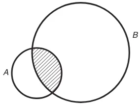
The intersection or product of A and B, written as A B, or simply AB, is the set of all elements that are common to A and B.

In terms of Venn diagrams, results of the above operations are shown in F igures 2.3(a) and 2.3(b) as sets having shaded areas.

If A B , sets A and B contain no common elements, and we call A and B disjoint. The symbol ‘ ’ shall be reserved to denote the union of two disjoint sets when it is advantageous to do so.

Ex ample 2. 2. Let A be the set of all men and B consist of all men and women over 18 years of age. Then the set A B consists of all men as well as all women over 18 years of age. The elements of A B are all men over 18 years of age.

Example 2.3.Let S be the space consisting of a real-line segment from 0 to 10 and let A and B be sets of the real-line segments from 1–7 and 3–9 respectively. Line segments belonging to andB are indicated in F igure 2.4. Let us note here that, by definition, a set and its complement are always disjoint.

The definitions of union and intersection can be directly generalized to those involving any arbitrary number (finite or countably infinite) of sets. Thus, the set

A B

(a) A B

A B

(b) A B

Figure 2. 3 (a) U nion and (b) intersection of sets A and B

A A

A B A B

B

0 2 4 6 8 10

Figure 2.4 Sets defined in Example 2.3

;

[

∪ ∩

\

[\

![). . .[

$!

$ )9

∪ ∩

(28)

stands for the set of all elements belonging to one or more of the sets Aj,

j 1, 2, . . . ,n. The intersection

is the set of all elements common to all Aj,j 1, 2, . . . ,n. The sets

Aj, j 1, 2, . . . , n, are disjoint if

Using Venn diagrams or analytical procedures, it is easy to verify that union and intersection operations are associative, commutative, and distributive; that is,

Clearly, we also have

(29)

The second relation in Equations (2.10) gives the union of two sets in terms of the union of two disjoint sets. As we will see, this representation is useful in probability calculations. The last two relations in Equations (2.10) are referred to as DeMorgan’s laws.

2. 2 S AM P L E S P A CE AN D P RO BA BILIT Y M E AS U RE

In probability theory, we are concerned with an experiment with an outcome depending on chance, which is called a random experiment. It is assumed that all possible distinct outcomes of a random experiment are known and that they are elements of a fundamental set known as the sample space. Each possible out-come is called a sample point, and an event is generally referred to as a subset of the sample space having one or more sample points as its elements.

It is important to point out that, for a given random experiment, the associated sample space is not unique and its construction depends upon the point of view adopted as well as the questions to be answered. F or example, 100 resistors are being manufactured by an industrial firm. Their values, owing to inherent inaccuracies in the manufacturing and measurement pro-cesses, may range from 99 to 101 . A measurement taken of a resistor is a random experiment for which the possible outcomes can be defined in a variety of ways depending upon the purpose for performing such an experiment. On

is considered acceptable, and unacceptable otherwise, it is adequate to define the sample space as one consisting of two elements: ‘acceptable’ and ‘unaccept-able’. On the other hand, from the viewpoint of another user, possible , 99.5–100 , 100–100.5 , and 100.5–101 . The sample space in this case has four sample points. F inally, if each possible reading is a possible outcome, the sample space is now a real line from 99 to 101 on the ohm scale; there is an uncountably infinite number of sample points, and the sample space is a nonenumerable set.

To illustrate that a sample space is not fixed by the action of performing the experiment but by the point of view adopted by the observer, consider an energy negotiation between the U nited States and another country. F rom the point of view of the U S government, success and failure may be looked on as the only possible outcomes. To the consumer, however, a set of more direct possible outcomes may consist of price increases and decreases for gasoline purchases.

The description of sample space, sample points, and events shows that they fit nicely into the framework of set theory, a framework within which the analysis of outcomes of a random experiment can be performed. All relations between outcomes or events in probability theory can be described by sets and set operations. Consider a space S of elements a, b, c, . . . , and with subsets

the one hand, if, for a given user, a resistor with resistance range of 99.9–100.1

(30)

A , B , C, . . . . Some of these corresponding sets and probability meanings are given in Table 2.1. As Table 2.1 shows, the empty set is considered an impossible event since no possible outcome is an element of the empty set. Also, by ‘occurrence of an event’ we mean that the observed outcome is an element of that set. F or example, event is said to occur if and only if the observed outcome is an element of or or both.

Example 2.4.Consider an experiment of counting the number of left-turning cars at an intersection in a group of 100 cars. The possible outcomes (possible numbers of left-turning cars) are 0, 1, 2, . . . , 100. Then, the sample space S is . Each element of S is a sample point or a possible out-come. The subset is the event that there are 50 or fewer cars turning left. The subset is the event that between 40 and 60 (inclusive) cars take left turns. The set is the event of 60 or fewer cars turning left. The set is the event that the number of left-turning cars is between 40 and 50 (inclusive). Let Events A and C are mutually exclusive since they cannot occur simultaneously. H ence, disjoint sets are mutually exclusive events in probability theory.

2.2.1 AXIOM S OF P ROBABILITY

We now introduce the notion of a probability function. G iven a random experi-ment, a finite number P(A) is assigned to every event A in the sample space S of all possible events. The number P(A) is a function of set A and is assumed to be defined for all sets in S. It is thus a set function, and P (A) is called the probability measure of A or simply the probability of A. It is assumed to have the following properties (axioms of probability):

Table 2.1 Corresponding statements in set theory and probability

Set theory Probability theory

( (

. . . ( . . . $

(. . . .

7

$

;

$

f* ! ). . . !**

f* ! ). . . 9*

f#* #!. . . 3*

[ \

f2* 2!. . . !**g

g

(31)

Axiom 1: P (A) 0 (nonnegative). Axiom 2: P (S) 1 (normed).

Axiom 3: for a countable collection of mutually exclusive events A1,A2, . . . inS,

These three axioms define a countably additive and nonnegative set function P(A), A S. As we shall see, they constitute a sufficient set of postulates from which all useful properties of the probability function can be derived. Let us give below some of these important properties.

F irst, P( ) 0. Since S and are disjoint, we see from Axiom 3 that

It then follows from Axiom 2 that

or

Second, if A C, then P (A) P (C). Since A C, one can write

where B is a subset of C and disjoint with A. Axiom 3 then gives

Since P (B) 0 as required by Axiom 1, we have the desired result. Third, given two arbitrary events A and B, we have

In order to show this, let us write A B in terms of the union of two mutually exclusive events. F rom the second relation in Equations (2.10), we write

.

![)[. . . $

$

$ )!!

; ;

!!;

; *

[ )!)

[

(32)

H ence, using Axiom 3,

F urthermore, we note

H ence, again using Axiom 3,

or

Substitution of this equation into Equation (2.13) yields Equation (2.12). Equation (2.12) can also be verified by inspecting the Venn diagram in F igure 2.5. The sum P (A) P (B) counts twice the events belonging to the shaded area AB. H ence, in computing P (A B), the probability associated with one AB must be subtracted from P (A) P (B), giving Equation (2.12) (see F igure 2.5).

The important result given by Equation (2.12) can be immediately general-ized to the union of three or more events. U sing the same procedure, we can show that, for arbitrary events A, B, and C,

A

B

Figure 2.5 Venn diagram for derivation of Equation (2.12)

)!4

[

[[

(33)

and, in the case of n events,

where Aj, j 1, 2, . . . ,n, are arbitrary events.

Example 2.5. Let us go back to Example 2.4 and assume that probabilities P (A), P (B), and P (C) are known. We wish to compute P(A B) and P(A C). Probability P(A C), the probability of having either 50 or fewer cars turn-ing left or between 80 to 100 cars turnturn-ing left, is simply P (A) P (C). This follows from Axiom 3, since A and C are mutually exclusive. H owever, P(A B), the probability of having 60 or fewer cars turning left, is found from

The information ine this probability

and we need the additional information, P (AB), which is the probability of having between 40 and 50 cars turning left.

With the statement of three axioms of probability, we have completed the mathematical description of a random experiment. It consists of three funda-mental constituents: a sample spaceS, a collection of eventsA, B,. . . , and the probability function P. These three quantities constitute a probability space associated with a random experiment.

2.2.2 ASSIGNM ENT OF P ROBABILITY

The axioms of probability define the properties of a probability measure, which are consistent with our intuitive notions. However, they do not guide us in assigning probabilities to various events. For problems in applied sciences, a natural way to assign the probability of an event is through the observation of relative frequency. Assuming that a random experiment is performed a large number of times, say n, then for any event A let nA be the number of occurrences of A in the n trials and define the ratio nA/n as the relative frequency of A. Under stable or statistical regularity conditions, it is expected that this ratio will tend to a unique limit as n becomes large. This limiting value of the relative frequency clearly possesses the properties required of the probability measure and is a natural candidate for the probability of A. This interpretation is used, for example, in saying that the

(34)

probability of ‘heads’ in flipping a coin is 1/2. The relative frequency approach to probability assignment is objective and consistent with the axioms stated in Section 2.2.1 and is one commonly adopted in science and engineering.

Another common but more subjective approach to probability assignment is that of relative likelihood. When it is not feasible or is impossible to perform an experiment a large number of times, the probability of an event may be assigned as a result of subjective judgement. The statement ‘there is a 40% probability of rain tomorrow’ is an example in this interpretation, where the number 0.4 is assigned on the basis of available information and professional judgement.

In most problems considered in this book, probabilities of some simple but basic events are generally assigned by using either of the two approaches. Other probabilities of interest are then derived through the theory of probability. Example 2.5 gives a simple illustration of this procedure where the probabilities of interest, P(A B) and P(A C), are derived upon assigning probabilities to simple events A, B, and C.

2.3 STATISTICAL INDEPENDENCE

Let us pose the following question: given individual probabilities P(A) and P (B) of two events A and B, what is P (AB), the probability that both A and B will occur? U pon little reflection, it is not difficult to see that the knowledge of P (A) and P(B) is not sufficient to determine P(AB) in general. This is so because P(AB) deals with joint behavior of the two events whereas P(A) and P(B) are probabilities associated with individual events and do not yield information on their joint behavior. Let us then consider a special case in which the occurrence or nonoccurrence of one does not affect the occurrence or nonoccurrence of the other. In this situation events A and B are called statistically independent or simply independent and it is formalized by D efinition 2.1.

D ef inition 2. 1. Two events A and B are said to be independent if and only if

To show that this definition is consistent with our intuitive notion of inde-pendence, consider the following example.

Ex ample 2. 6. In a large number of trials of a random experiment, let nA and

nB be, respectively, the numbers of occurrences of two outcomes A and B, and let nAB be the number of times both A and B occur. U sing the relative frequency interpretation, the ratios nA/n and nB/n tend to P(A) and P(B), respectively, as n becomes large. Similarly, nA B/n tends to P(AB). Let us now confine our atten-tion to only those outcomes in which A is realized. If A and B are independent,

(35)

we expect that the ratio nA B/nA also tends to P(B) as nA becomes large. The independence assumption then leads to the observation that

This then gives

or, in the limit as n becomes large,

which is the definition of independence introduced above.

Example 2.7. In launching a satellite, the probability of an unsuccessful launch is q. What is the probability that two successive launches are unsuccess-ful? Assuming that satellite launchings are independent events, the answer to the above question is simply q2. One can argue that these two events are not really completely independent, since they are manufactured by using similar processes and launched by the same launcher. It is thus likely that the failures of both are attributable to the same source. H owever, we accept this answer as reasonable because, on the one hand, the independence assumption is accept-able since there are a great deal of unknowns involved, any of which can be made accountable for the failure of a launch. On the other hand, the simplicity of computing the joint probability makes the independence assumption attract-ive. In physical problems, therefore, the independence assumption is often made whenever it is considered to be reasonable.

Care should be exercised in extending the concept of independence to more than two events. In the case of three events, A1,A2, andA3, for example, they are mutually independent if and only if

and

Equation (2.18) is required because pairwise independence does not generally lead to mutual independence. Consider, for example, three events A1,A2, and

A3defined by

$- $- $6- $-!)4 )!1

!)4 !)4 )!2

(36)

where B1,B2, andB3 are mutually exclusive, each occurring with probability1₄. It is easy to calculate the following:

We see that Equation (2.17) is satisfied for every j and k in this case, but Equation (2.18) is not. In other words, events A1, A2, and A3 are pairwise independent but they are not mutually independent.

In general, therefore, we have D efinition 2.2 for mutual independence of nevents.

D ef inition 2. 2. Events A1,A2, . . . ,An are mutually independent if and only if, with k1,k2, . . . ,km being any set of integers such that 1 k1 < k2 . . . < km n and m 2, 3, . . . , n,

The total number of equations defined by Equation (2.19) is 2n _n _1. Example 2.8.Problem: a system consisting of five components is in working order only when each component is functioning (‘good’). Let Si,i 1, . . . , 5, be the event that the ith component is good and assume P(Si) pi. What is the probability q that the system fails?

Answer: assuming that the five components perform in an independent manner, it is easier to determine q through finding the probability of system success p. We have from the statement of the problem

Equation (2.19) thus gives, due to mutual independence of S1,S2, . . . ,S5,

H ence,

! ![) ! )

!

)

) 4

!

)

!) ![) \ ![4 ! !

#

!4 )4

!

#

!)4 ![) \ ![4 \ )[4 ; *

-!-). . .- -!-). . .- )!"

!)4#9

!). . .9 !)4#9 ))*

(37)

An expression for q may also be obtained by noting that the system fails if any one or more of the five components fail, or

whereSi is the complement of Si and represents a bad ith component. Clearly, . Since events 1, . . . , 5, are not mutually exclusive, the calculation of q with use of Equation (2.22) requires the use of Equation (2.15). Another approach is to write the unions in Equation (2.22) in terms of unions of mutually exclusive events so that Axiom 3 (Section 2.2.1) can be directly utilized. The result is, upon applying the second relation in Equations (2.10),

where the ‘ ’ signs are replaced by ‘ ’ signs on the right-hand side to stress the fact that they are mutually exclusive events. Axiom 3 then leads to

and, using statistical independence,

Some simple algebra will show that this result reduces to Equation (2.21).

Let us mention here that probability p is called the reliability of the system in systems engineering.

2.4 CONDITIONAL PROBABILITY

The concept of conditional probability is a very useful one. G iven two events A and B associated with a random experiment, probability is defined as the conditional probability of A, given that B has occurred. Intuitively, this probability can be interpreted by means of relative frequencies described in Example 2.6, except that events A and B are no longer assumed to be independ-ent. The number of outcomes where both A and B occur is nA B. H ence, given that event B has occurred, the relative frequency of A is then nA B/nB. Thus we have, in the limit as nB becomes large,

This relationship leads to D efinition 2.3.

![)[4[#[9 )))

$!

![)[4[#[9!!)!)4!)4#!)4#9

[

! !) !)4 !)4# !)4#9

! ! !! ) !)! 4 !)4! # !)4#! 9

))4

j$

j

(38)

D ef inition 2 . 3. The conditional probability of A given that B has occurred is given by

D efinition 2.3 is meaningless if P (B) 0.

It is noted that, in the discussion of conditional probabilities, we are dealing with a contracted sample space in which B is known to have occurred. In other words, B replaces S as the sample space, and the conditional probability P(A B) is found as the probability of A with respect to this new sample space.

In the event that A and B are independent, it implies that the occurrence of B has no effect on the occurrence or nonoccurrence of A. We thus expect

and Equation (2.24) gives

or

which is precisely the definition of independence.

It is also important to point out that conditional probabilities are probabilities (i.e. they satisfy the three axioms of probability). Using Equation (2.24), we see that the first axiom is automatically satisfied. For the second axiom we need to show that

This is certainly true, since

As for the third axiom, if A1,A2, . . . are mutually exclusive, then A1B, A2B, . . . are also mutually exclusive. H ence,

6* ))#

j

j$$

j !

j

!

![)[. . .j

![)[. . .

!

)

(39)

and the third axiom holds.

The definition of conditional probability given by Equation (2.24) can be used not only to compute conditional probabilities but also to compute joint probabilities, as the following examples show.

Example 2.9.Problem: let us reconsider Example 2.8 and ask the following question: what is the conditional probability that the first two components are good given that (a) the first component is good and (b) at least one of the two is good?

Answer: the event S1S2 means both are good components, and S1 S2 is the event that at least one of the two is good. Thus, for question (a) and in view of Equation (2.24),

This result is expected since S1 and S2 are independent. Intuitively, we see that this question is equivalent to one of computing P(S2).

F or question (b), we have

Example 2.10. Problem: in a game of cards, determine the probability of drawing, without replacement, two aces in succession.

Answer: let A1be the event that the first card drawn is an ace, and similarly for A2. We wish to compute P(A1A2). F rom Equation (2.24) we write

N ow, and (there are 51 cards left and three of them are aces). Therefore,

!)!

!

!)

!

!)

!

)

!)j![) !)![)

![)

/!) ![)$!) 5

!)j![) !)

![)

!)

! ) !)

!)

!) !)

!) )j!! ))9 !$#C9) )j!$4C9!

!)

4 9!

# 9)

!

(40)

Equation (2.25) is seen to be useful for finding joint probabilities. Its exten-sion to more than two events has the form

where P(Ai) > 0 for all i. This can be verified by successive applications of Equation (2.24).

In another direction, let us state a useful theorem relating the probability of an event to conditional probabilities.

Theorem 2. 1: t heorem of t ot a l probabilit y . Suppose that events B1,B2, . . . , and

Bn are mutually exclusive and exhaustive (i.e. S B1 B2 Bn). Then, for an arbitrary event A,

Proof of Theorem 2.1:referring to the Venn diagram in F igure 2.6, we can clearly write A as the union of mutually exclusive events AB1,AB2, . . . ,ABn (i.e.

). H ence,

which gives Equation (2.27) on application of the definition of conditional probability.

AB1

B₁

B₂

B3

B5

B₄ AB3

AB₂ AB4

AB₅

S

A

Figure 2.6 Venn diagram associated with total probability

!). . . !)j!4j!). . .j!). . . ! ))3

j!! j)) j

$!

j$$

))1

!)

(41)

The utility of this result rests with the fact that the probabilities in the sum in Equation (2.27) are often more readily obtainable than the probability of A itself. Example 2.11. Our interest is in determining the probability that a critical level of peak flow rate is reached during storms in a storm-sewer system on the basis of separate meteorological and hydrological measurements.

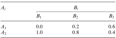
Let Bi,i 1, 2, 3, be the different levels (low, medium, high) of precipitation caused by a storm and let 1, 2, denote, respectively, critical and non-critical levels of peak flow rate. Then probabilities P(Bi) can be estimated from meteorological records and can be estimated from runoff analysis. Since B1,B2, and B3 constitute a set of mutually exclusive and exhaustive events, the desired probability, P(A1), can be found from

Assume the following information is available:

and that are as shown in Table 2.2. The value of P (A1) is given by

Let us observe that in Table 2.2, the sum of the probabilities in each column is 1.0 by virtue of the conservation of probability. There is, however, no such requirement for the sum of each row.

A useful result generally referred to as Bayes’ theorem can be derived based on the definition of conditional probability. Equation (2.24) permits us to write

and

Since we have Theorem 2.2.

Table 2.2 Probabilities for Example 2.11

0.0 0.2 0.6

1.0 0.8 0.4

$$

$j$

! !j!! !j)) !j44

! *9 ) *4 4 *) $j$

! **9 *)*4 *3*) *!2

j

j $$

$j$

$

! ) 4

!

(42)

Theorem 2. 2: Bay es’ t heorem. Let A and B be two arbitrary events with 0 and 0. Then:

Combining this theorem with the total probability theorem we have a useful consequence:

for any i where events Bj represent a set of mutually exclusive and exhaustive events.

The simple result given by Equation (2.28) is called Bayes’ theorem after the English philosopher Thomas Bayes and is useful in the sense that it permits us to evaluate a posteriori probability in terms of a priori information P(B) and , as the following examples illustrate.

Example 2.12. Problem: a simple binary communication channel carries messages by using only two signals, say 0 and 1. We assume that, for a given binary channel, 40% of the time a 1 is transmitted; the probability that a transmitted 0 is correctly received is 0.90, and the probability that a transmitted 1 is correctly received is 0.95. D etermine (a) the probability of a 1 being received, and (b) given a 1 is received, the probability that 1 was transmitted.

Answer: let

event that 1 is transmitted event that 0 is transmitted event that 1 is received event that 0 is received

The information given in the problem statement gives us

and these are represented diagrammatically in F igure 2.7.

F or part (a) we wish to find P(B). Since A andA are mutually exclusive and exhaustive, it follows from the theorem of total probability [Equation (2.27)] $6 $6

j j

))2

j j

$!

j$$

))"

j$

$

*#

j *"9

j *"*

(43)

that

The probability of interest in part (b) is and this can be found using Bayes’ theorem [Equation (2.28)]. It is given by:

It is worth mentioning that P(B) in this calculation is found by means of the total probability theorem. H ence, Equation (2.29) is the one actually used here in finding In fact, probability P(A) in Equation (2.28) is often more conveniently found by using the total probability theorem.

Example 2.13.Problem: from Example 2.11, determine the probabil-ity that a noncritical level of peak flow rate will be caused by a medium-level storm.

Answer: from Equations (2.28) and (2.29) we have

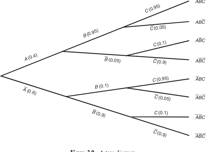
In closing, let us introduce the use of tree diagrams for dealing with more complicated experiments with ‘limited memory’. Consider again Example 2.12

0.4

0.6

0.95

0.9 0.0₅

0.1

B

A B

A

Figure 2.7 Probabilities associated with a binary channel, for Example 2.12

j j *"9*# *!*3 *##

$

j

*"9*#

*## *234

j$

)j)$

)j)

)j)) )

)j))

)j!! )j)) )j44

*2*4

(44)

by adding a second stage to the communication channel, with F igure 2.8 showing all the associated probabilities. We wish to determine P (C), the prob-ability of receiving a 1 at the second stage.

Tree diagrams are useful for determining the behavior of this system when the system has a ‘one-stage’ memory; that is, when the outcome at the second stage is dependent only on what has happened at the first stage and not on outcomes at stages prior to the first. M athematically, it follows from this property that

The properties described above are commonly referred to as M arkovian properties. M arkov processes represent an important class of probabilistic process that are studied at a more advanced level.

Suppose that Equations (2.30) hold for the system described in F igure 2.8. The tree diagram gives the flow of conditional probabilities originating from the source. Starting from the transmitter, the tree diagram for this problem has the appearance shown in F igure 2.9. The top branch, for example, leads to the probability of the occurrence of event ABC, which is, according to Equations (2.26) and (2.30),

The probability of C is then found by summing the probabilities of all events that end with C. Thus,

0.4

0.6

0.95

0.9 0.9

0.95

0.1 0.1

0.05 _0.0

5

A B

B

C

C A

Figure 2.8 A two-stage binary channel

j j j )4*

jj jj

*#*"9*"9 *43!

*"9*"9*# *!**9*# *"9*!*3 *!*"*3

(45)

REFERENCE

Todhunter, I., 1949, A History of the Mathematical Theory of Probability from the Time of Pascal to Laplace, Chelsea, N ew York.

FURTHER READING

M ore accounts of early development of probability theory related to gambling can be found in

D avid, F .N ., 1962, Games, Gods, and Gambling, H afner, N ew York.

PROBLEMS

2.1 Let A, B, and C be arbitrary sets. D etermine which of the following relations are correct and which are incorrect:

(a) (b) (c) (d)

ABC

ABC ABC

A (0.4)

B (0.95)

C (0.95)

A (0.6₎

B (0.9₎

C (0.9) C (0.05)

C (0.1)

C (0.9)

C (0.95)

C (0.05)

C (0.1)

B (0.05)

B (0.1)

Figure 2.9 A tree diagram

[$

[

(46)

(e) (f)

2.2 The second relation in Equations (2.10) expresses the union of two sets as the union of two disjoint sets (i.e. ). Express in terms of the union of disjoint sets where A, B, and C are arbitrary sets.

2.3 Verify D eM organ’s laws, given by the last two equations of Equations (2.10).

2.4 Let D etermine

elements of the following sets: (a)

2.5 R epeat Problem 2.4 if and

2.6 D raw Venn diagrams of events A and B representing the following situations: (a) A and B are arbitrary. (c) Only one occurs. (d) At least one occurs.

(e) A occurs and either B or C occurs but not both. (f) B and C occur, but A does not occur.

(g) Two or more occur. (h) At most two occur. (i) All three occur.

2.8 Events A, B, and C are independent, with

D etermine the following probabilities in terms of a, b, and c: (a)

(b) (c) (d)

2.9 An engineering system has two components. Let us define the following events: A : first component is good;A: first component is defective.

B : second component is good;B: second component is defective: D escribe the following events in terms of A,A, B, andB: (a) At least one of the components is good.

(b) One is good and one is defective.

(47)

2.10 F or the two components described in Problem 2.9, tests have produced the follow-ing result:

D etermine the probability that: (a) The second component is good. (b) At least one of the components is good.

(c) The first component is good given that the second is good.

(d) The first component is good given that at most one component is good. F or the two eventsAandB:

(e) Are they independent? Verify your answer. (f) Are they mutually exclusive? Verify your answer.

2.11 A satellite can fail for many possible reasons, two of which are computer failure and engine failure. F or a given mission, it is known that:

The probability of engine failure is 0.008. The probability of computer failure is 0.001.

G iven engine failure, the probability of satellite failure is 0.98. G iven computer failure, the probability of satellite failure is 0.45.

G iven any other component failure, the probability of satellite failure is zero. (a) D etermine the probability that a satellite fails.

(b) D etermine the probability that a satellite fails and is due to engine failure.

(c) Assume that engines in different satellites perform independently. G iven a satellite has failed as a result of engine failure, what is the probability that the same will happen to another satellite?

2.12 Verify Equation (2.14). 2.13 Show that, for arbitrary events

This is known as Boole’s inequality.

2.14 A box contains 20 parts, of which 5 are defective. Two parts are drawn at random from the box. What is the probability that:

(a) Both are good? (b) Both are defective?

(c) One is good and one is defective?

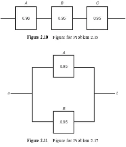
2.15 An automobile braking device consists of three subsystems, all of which must work for the device to work. These systems are an electronic system, a hydraulic system, and a mechanical activator. In braking, the reliabilities (probabilities of success) of these units are 0.96, 0.95, and 0.95, respectively. Estimate the system reliability assuming that these subsystems function independently.

Comment: systems of this type can be graphically represented as shown in F igure 2.10, in which subsystems A (electronic system), B (hydraulic system), and

*2 j *29 j *19

!). . .

(48)

C (mechanical activator) are arranged in series. Consider the path as the ‘path to success’. A breakdown of any or all of A, B, or C will block the path from

atob.

2.16 A spacecraft has 1000 components in series. If the required reliability of the spacecraft is 0.9 and if all components function independently and have the same reliability, what is the required reliability of each component?

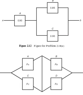
2.17 Automobiles are equipped with redundant braking circuits; their brakes fail only when all circuits fail. Consider one with two redundant braking circuits, each having a reliability of 0.95. D etermine the system reliability assuming that these circuits act independently.

Comment: systems of this type are graphically represented as in F igure 2.11, in which the circuits (A and B) have a parallel arrangement. The path to success is broken only when breakdowns of both A and B occur.

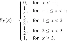
2.18 On the basis of definitions given in Problems 2.15 and 2.17 for series and parallel arrangements of system components, determine reliabilities of the systems described by the block diagrams as follows.

(a) The diagram in F igure 2.12. (b) The diagram in F igure 2.13.

a b

A

0.96

B

0.95

C

0.95

Figure 2.10 F igure for Problem 2.15

A

B

a b

0.95

Figure 2.11 F igure for Problem 2.17

(49)

2.19 A rifle is fired at a target. Assuming that the probability of scoring a hit is 0.9 for each shot and that the shots are independent, compute the probability that, in order to score a hit:

(a) It takes more than two shots.

(b) The number of shots required is between four and six (inclusive).

2.20 Events A and B are mutually exclusive. Can they also be independent? Explain. 2.21 Let

(a) A and B are independent? (b) A and B are mutually exclusive?

2.22 Let Is it possible to determine P(A) and P (B)? Answer the same question if, in addition:

(a) A and B are independent. (b) A and B are mutually exclusive.

a b

A

B

C 0.90

0.90 0.85

Figure 2.12 F igure for Problem 2.18(a)

a b

A B

C D

p_A

pC pD

p_B

Figure 2.13 F igure for Problem 2.18(b)

$*# [$*1 , $ 0

(50)

2.23 Events A and B are mutually exclusive. D etermine which of the following relations are true and which are false:

R epeat the above if events A and B are independent.

2.24 On a stretch of highway, the probability of an accident due to human error in any given minute is 10 5_{, and the probability of an accident due to mechanical} break-down in any given minute is 10 7_{. Assuming that these two causes are independent:} (a) F ind the probability of the occurrence of an accident on this stretch of highway

during any minute.

(b) In this case, can the above answer be approximated by P(accident due to human error) P(accident due to mechanical failure)? Explain.

(c) If the events in succeeding minutes are mutually independent, what is the probability that there will be no accident at this location in a year?

2.25 R apid transit trains arrive at a given station every five minutes and depart after stopping at the station for one minute to drop off and pick up passengers. Assum-ing trains arrive every hour on the hour, what is the probability that a passenger will be able to board a train immediately if he or she arrives at the station at a random instant between 7:54 a.m. and 8:06 a.m.?

2.26 A telephone call occurs at random in the interval (0,t). Let T be its time of occurrence. D etermine, where 0

(a) (b)

2.27 F or a storm-sewer system, estimates of annual maximum flow rates (AM F R ) and their likelihood of occurrence [assuming that a maximum of 12 cfs (cubic feet per second) is possible] are given as follows:

Event

2.28 At a major and minor street intersection, one finds that, out of every 100 gaps on the major street, 65 are acceptable, that is, large enough for a car arriving on the minor street to cross. When a vehicle arrives on the minor street:

(a) What is the probability that the first gap is not an acceptable one? (b) What is the probability that the first two gaps are both unacceptable? (c) The first car has crossed the intersection. What is the probability that the

second will be able to cross at the very next gap?

(51)

2.29 A machine part may be selected from any of three manufacturers with probabilities The probabilities that it will function properly during a specified period of time are 0.2, 0.3, and 0.4, respectively, for the three manufacturers. D etermine the probability that a randomly chosen machine part will function properly for the specified time period.

2.30 Consider the possible failure of a transportation system to meet demand during rush hour.

(a) D etermine the probability that the system will fail if the probabilities shown in Table 2.3 are known.

(b) If system failure was observed, find the probability that a ‘medium’ demand level was its cause.

2.31 A cancer diagnostic test is 95% accurate both on those who have cancer and on those who do not. If 0.005 of the population actually does have cancer, compute the probability that a particular individual has cancer, given that the test indicates he or she has cancer.

2.32 A quality control record panel of transistors gives the results shown in Table 2.4 when classified by manufacturer and quality.

Let one transistor be selected at random. What is the probability of it being: (a) F rom manufacturer A and with acceptable quality?

(b) Acceptable given that it is from manufacturer C? (c) F rom manufacturer B given that it is marginal?

2.33 Verify Equation (2.26) for three events.

2.34 In an elementary study of synchronized traffic lights, consider a simple four-light system. Suppose that each light is red for 30 seconds of a 50-second cycle, and suppose

and

Table 2.3 Probabilities of demand levels and of system

failures for the given demand level, for Problem 2.30 D emand level P(level) P(system failure level)

Low 0.6 0

M edium 0.3 0.1

H igh 0.1 0.5

Table 2.4 Quality control results, for Problem 2.32

M anufacturer Quality

Acceptable M arginal U nacceptable Total

A 128 10 2 140

B 97 5 3 105

C 110 5 5 120

!*)9)*9* 4*)9

j

$!j$ *!9

(52)

for j 1, 2, 3, where Sjis the event that a driver is stopped by the jth light. We assume a ‘one-light’ memory for the system. By means of the tree diagram, determine the probability that a driver:

(a) Will be delayed by all four lights.

(b) Will not be delayed by any of the four lights. (c) Will be delayed by at most one light.

(53)

(54)

3 R andom Variables and Probability

D istributions

We have mentioned that our interest in the study of a random phenomenon is in the statements we can make concerning the events that can occur, and these statements are made based on probabilities assigned to simple outcomes. Basic concepts have been developed in Chapter 2, but a systematic and unified procedure is needed to facilitate making these statements, which can be quite complex. One of the immedi-ate steps that can be taken in this unifying attempt is to require that each of the possible outcomes of a random experiment be represented by a real number. In this way, when the experiment is performed, each outcome is identified by its assigned real number rather than by its physical description. For example, when the possible outcomes of a random experiment consist of success and failure, we arbitrarily assign the number one to the event ‘success’ and the number zero to the event ‘failure’. The associated sample space has now 1, 0 as its sample points instead of success and failure, and the statement ‘the outcome is 1’ means ‘the outcome is success’.

This procedure not only permits us to replace a sample space of arbitrary elements by a new sample space having only real numbers as its elements but also enables us to use arithmetic means for probability calculations. F urther-more, most problems in science and engineering deal with quantitative meas-ures. Consequently, sample spaces associated with many random experiments of interest are already themselves sets of real numbers. The real-number assign-ment procedure is thus a natural unifying agent. On this basis, we may intro-duce a variable , which is used to represent real numbers, the values of which are determined by the outcomes of a random experiment. This leads to the notion of a random variable, which is defined more precisely below.

3.1 RANDOM VARIABLES

Consider a random experiment to which the outcomes are elements of sample space in the underlying probability space. In order to construct a model for

f g