Probability Statistics for Engineers Scientists

(1)

Probability & Statistics for

Engineers & Scientists

N I N T H

E D I T I O N

Ronald E. Walpole

Roanoke College

Raymond H. Myers

Virginia Tech

Sharon L. Myers

Radford University

Keying Ye

University of Texas at San Antonio

(2)

Chapter 4

Mathematical Expectation

4.1 Mean of a Random Variable

In Chapter 1, we discussed the sample mean, which is the arithmetic mean of the data. Now consider the following. If two coins are tossed 16 times and X is the number of heads that occur per toss, then the values ofX are 0, 1, and 2. Suppose that the experiment yields no heads, one head, and two heads a total of 4, 7, and 5 times, respectively. The average number of heads per toss of the two coins is then

(0)(4) + (1)(7) + (2)(5)

16 = 1.06.

This is an average value of the data and yet it is not a possible outcome of{0,1,2}. Hence, an average is not necessarily a possible outcome for the experiment. For instance, a salesman’s average monthly income is not likely to be equal to any of his monthly paychecks.

Let us now restructure our computation for the average number of heads so as to have the following equivalent form:

(0) ₄

16

+ (1) ₇

16

+ (2) ₅

16

= 1.06.

The numbers 4/16, 7/16, and 5/16 are the fractions of the total tosses resulting in 0, 1, and 2 heads, respectively. These fractions are also the relative frequencies for the different values ofX in our experiment. In fact, then, we can calculate the mean, or average, of a set of data by knowing the distinct values that occur and their relative frequencies, without any knowledge of the total number of observations in our set of data. Therefore, if 4/16, or 1/4, of the tosses result in no heads, 7/16 of the tosses result in one head, and 5/16 of the tosses result in two heads, the mean number of heads per toss would be 1.06 no matter whether the total number of tosses were 16, 1000, or even 10,000.

This method of relative frequencies is used to calculate the average number of heads per toss of two coins that we might expect in the long run. We shall refer to this average value as the mean of the random variable X or the mean of the probability distribution of X and write it asµxor simply asµwhen it is

(3)

112 Chapter 4 Mathematical Expectation

clear to which random variable we refer. It is also common among statisticians to refer to this mean as the mathematical expectation, or the expected value of the random variableX, and denote it asE(X).

Assuming that 1 fair coin was tossed twice, we find that the sample space for our experiment is

S={HH, HT, T H, T T}.

Since the 4 sample points are all equally likely, it follows that

P(X = 0) =P(T T) =1

4, P(X= 1) =P(T H) +P(HT) = 1 2,

and

P(X = 2) =P(HH) =1 4,

where a typical element, say T H, indicates that the first toss resulted in a tail followed by a head on the second toss. Now, these probabilities are just the relative frequencies for the given events in the long run. Therefore,

µ=E(X) = (0)

1 4

+ (1)

1 2

+ (2)

1 4

= 1.

This result means that a person who tosses 2 coins over and over again will, on the average, get 1 head per toss.

The method described above for calculating the expected number of heads per toss of 2 coins suggests that the mean, or expected value, of any discrete random variable may be obtained by multiplying each of the valuesx1, x2, . . . , xn

of the random variableX by its corresponding probabilityf(x1), f(x2), . . . , f(xn)

and summing the products. This is true, however, only if the random variable is discrete. In the case of continuous random variables, the definition of an expected value is essentially the same with summations replaced by integrations.

Definition 4.1: _Let _X _{be a random variable with probability distribution} _f₍_x_{). The} _mean_{, or}

expected value, ofX is

µ=E(X) =

x

xf(x)

ifX is discrete, and

µ=E(X) = ∞

−∞

xf(x)dx

ifX is continuous.

(4)

4.1 Mean of a Random Variable 113

However, the mean is usually understood as a “center” value of the underlying distribution if we use the expected value, as in Definition 4.1.

Example 4.1: A lot containing 7 components is sampled by a quality inspector; the lot contains 4 good components and 3 defective components. A sample of 3 is taken by the inspector. Find the expected value of the number of good components in this sample.

Solution:Let X represent the number of good components in the sample. The probability distribution ofX is

f(x) = 4

x

3 3−x

7 3

, x= 0,1,2,3.

Simple calculations yield f(0) = 1/35, f(1) = 12/35, f(2) = 18/35, and f(3) = 4/35. Therefore,

µ=E(X) = (0) ₁

35

+ (1) ₁₂

35

+ (2) ₁₈

35

+ (3) ₄

35

=12 7 = 1.7.

Thus, if a sample of size 3 is selected at random over and over again from a lot of 4 good components and 3 defective components, it will contain, on average, 1.7 good components.

Example 4.2: A salesperson for a medical device company has two appointments on a given day. At the first appointment, he believes that he has a 70% chance to make the deal, from which he can earn $1000 commission if successful. On the other hand, he thinks he only has a 40% chance to make the deal at the second appointment, from which, if successful, he can make $1500. What is his expected commission based on his own probability belief? Assume that the appointment results are independent of each other.

Solution:First, we know that the salesperson, for the two appointments, can have 4 possible commission totals: $0, $1000, $1500, and $2500. We then need to calculate their associated probabilities. By independence, we obtain

f($0) = (1−0.7)(1−0.4) = 0.18, f($2500) = (0.7)(0.4) = 0.28, f($1000) = (0.7)(1−0.4) = 0.42, andf($1500) = (1−0.7)(0.4) = 0.12.

Therefore, the expected commission for the salesperson is

E(X) = ($0)(0.18) + ($1000)(0.42) + ($1500)(0.12) + ($2500)(0.28) = $1300.

(5)

Example 4.3: LetX be the random variable that denotes the life in hours of a certain electronic device. The probability density function is

f(x) =

₂₀_,₀₀₀

x3 , x >100,

0, elsewhere.

Find the expected life of this type of device.

Solution:Using Definition 4.1, we have

µ=E(X) = ∞

100

x20,000 x3 dx=

∞

100

20,000

x2 dx= 200.

Therefore, we can expect this type of device to last, on average, 200 hours. Now let us consider a new random variable g(X), which depends on X; that is, each value of g(X) is determined by the value of X. For instance,g(X) might be X2 _{or 3}_X ₋_{1, and whenever}_X _{assumes the value 2,} _g₍_X_{) assumes the value} g(2). In particular, ifXis a discrete random variable with probability distribution

f(x), forx=−1,0,1,2, andg(X) =X2_{, then}

P[g(X) = 0] =P(X = 0) =f(0),

P[g(X) = 1] =P(X =−1) +P(X = 1) =f(−1) +f(1), P[g(X) = 4] =P(X = 2) =f(2),

and so the probability distribution of g(X) may be written

g(x) 0 1 4

P[g(X) =g(x)] f(0) f(−1) +f(1) f(2)

By the definition of the expected value of a random variable, we obtain

µg(X)=E[g(x)] = 0f(0) + 1[f(−1) +f(1)] + 4f(2)

= (−1)2f(−1) + (0)2f(0) + (1)2f(1) + (2)2f(2) =

x

g(x)f(x).

This result is generalized in Theorem 4.1 for both discrete and continuous random variables.

Theorem 4.1: Let X be a random variable with probability distribution f(x). The expected value of the random variableg(X) is

µg(X)=E[g(X)] =

x

g(x)f(x)

µg(X)=E[g(X)] =

∞

−∞

g(x)f(x)dx

(6)

4.1 Mean of a Random Variable 115

Example 4.4: Suppose that the number of cars X that pass through a car wash between 4:00

P.M.and 5:00P.M.on any sunny Friday has the following probability distribution:

x 4 5 6 7 8 9 by the manager. Find the attendant’s expected earnings for this particular time period.

Solution:By Theorem 4.1, the attendant can expect to receive

E[g(X)] =E(2X−1) =

Example 4.5: LetX be a random variable with density function

f(x) =

Solution:By Theorem 4.1, we have

E(4X+ 3) =

We shall now extend our concept of mathematical expectation to the case of two random variablesX andY with joint probability distributionf(x, y).

Definition 4.2: _Let_X_and_Y _{be random variables with joint probability distribution}_f₍_{x, y}_{). The}

mean, or expected value, of the random variableg(X, Y) is

µg(X,Y)=E[g(X, Y)] =

ifX andY are discrete, and

µg(X,Y)=E[g(X, Y)] =

ifX andY are continuous.

(7)

Example 4.6: LetX andY be the random variables with joint probability distribution indicated in Table 3.1 on page 96. Find the expected value of g(X, Y) =XY. The table is reprinted here for convenience.

x Row

Solution:By Definition 4.2, we write

E(XY) =

Example 4.7: FindE(Y /X) for the density function

f(x, y) =

_x₍₁₊₃_y2 )

4 , 0< x <2, 0< y <1,

0, elsewhere.

Solution:We have

E

where g(x) is the marginal distribution ofX. Therefore, in calculatingE(X) over a two-dimensional space, one may use either the joint probability distribution of

X andY or the marginal distribution ofX. Similarly, we define

E(Y) =

(8)

/ /

Exercises 117

Exercises

4.1 The probability distribution ofX, the number of imperfections per 10 meters of a synthetic fabric in con-tinuous rolls of uniform width, is given in Exercise 3.13 on page 92 as

x 0 1 2 3 4

f(x) 0.41 0.37 0.16 0.05 0.01 Find the average number of imperfections per 10 me-ters of this fabric.

4.2 The probability distribution of the discrete ran-dom variableX is

f(x) =

4.3 Find the mean of the random variable T repre-senting the total of the three coins in Exercise 3.25 on page 93.

4.4 A coin is biased such that a head is three times as likely to occur as a tail. Find the expected number of tails when this coin is tossed twice.

4.5 In a gambling game, a woman is paid $3 if she draws a jack or a queen and $5 if she draws a king or an ace from an ordinary deck of 52 playing cards. If she draws any other card, she loses. How much should she pay to play if the game is fair?

4.6 An attendant at a car wash is paid according to the number of cars that pass through. Suppose the probabilities are 1/12, 1/12, 1/4, 1/4, 1/6, and 1/6, respectively, that the attendant receives $7, $9, $11, $13, $15, or $17 between 4:00 P.M.and 5:00 P.M. on any sunny Friday. Find the attendant’s expected earn-ings for this particular period.

4.7 By investing in a particular stock, a person can make a proﬁt in one year of $4000 with probability 0.3 or take a loss of $1000 with probability 0.7. What is this person’s expected gain?

4.8 Suppose that an antique jewelry dealer is inter-ested in purchasing a gold necklace for which the prob-abilities are 0.22, 0.36, 0.28, and 0.14, respectively, that she will be able to sell it for a profit of $250, sell it for a profit of $150, break even, or sell it for a loss of $150. What is her expected profit?

4.9 A private pilot wishes to insure his airplane for $200,000. The insurance company estimates that a to-tal loss will occur with probability 0.002, a 50% loss with probability 0.01, and a 25% loss with probability

0.1. Ignoring all other partial losses, what premium should the insurance company charge each year to re-alize an average proﬁt of $500?

4.10 Two tire-quality experts examine stacks of tires and assign a quality rating to each tire on a 3-point scale. LetX denote the rating given by expertA and

Y denote the rating given by B. The following table gives the joint distribution forX andY.

y

4.11 The density function of coded measurements of the pitch diameter of threads of a ﬁtting is

f(x) =

₄

π(1+x2₎, 0< x <1,

0, elsewhere.

Find the expected value ofX.

4.12 If a dealer’s proﬁt, in units of $5000, on a new automobile can be looked upon as a random variable

X having the density function

f(x) =

2(1−x), 0< x <1,

0, elsewhere,

ﬁnd the average proﬁt per automobile.

4.13 The density function of the continuous random variableX, the total number of hours, in units of 100 hours, that a family runs a vacuum cleaner over a pe-riod of one year, is given in Exercise 3.7 on page 92 as

Find the average number of hours per year that families run their vacuum cleaners.

4.14 Find the proportionXof individuals who can be expected to respond to a certain mail-order solicitation ifX has the density function

f(x) =

₂₍_x₊₂₎

5 , 0< x <1,

(9)

/ /

4.15 Assume that two random variables (X, Y) are uniformly distributed on a circle with radius a. Then the joint probability density function is

f(x, y) =

4.16 Suppose that you are inspecting a lot of 1000 light bulbs, among which 20 are defectives. You choose two light bulbs randomly from the lot without replace-ment. Let

Find the probability that at least one light bulb chosen is defective. [Hint: ComputeP(X1+X2= 1).]

4.17 LetX be a random variable with the following probability distribution:

x −3 6 9

f(x) 1/6 1/2 1/3

Findµg(X), whereg(X) = (2X+ 1)2.

4.18 Find the expected value of the random variable

g(X) =X2, where X has the probability distribution of Exercise 4.2.

4.19 A large industrial ﬁrm purchases several new word processors at the end of each year, the exact num-ber depending on the frequency of repairs in the previ-ous year. Suppose that the number of word processors,

X, purchased each year has the following probability distribution:

x 0 1 2 3

f(x) 1/10 3/10 2/5 1/5

If the cost of the desired model is $1200 per unit and at the end of the year a refund of 50X2 dollars will be issued, how much can this ﬁrm expect to spend on new word processors during this year?

4.20 A continuous random variableXhas the density function

f(x) =

_e−x_, _{x >}₀_,

0, elsewhere.

Find the expected value ofg(X) =e2X/3_.

4.21 What is the dealer’s average proﬁt per auto-mobile if the proﬁt on each autoauto-mobile is given by

g(X) =X2_{, where}_X _{is a random variable having the}

density function of Exercise 4.12?

4.22 The hospitalization period, in days, for patients following treatment for a certain type of kidney disor-der is a random variableY =X+ 4, whereX has the

Find the average number of days that a person is hos-pitalized following treatment for this disorder.

4.23 Suppose thatX andY have the following joint probability function:

4.24 Referring to the random variables whose joint probability distribution is given in Exercise 3.39 on page 105,

(a) ﬁndE(X2Y −2XY); (b) ﬁndµX−µY.

4.25 Referring to the random variables whose joint probability distribution is given in Exercise 3.51 on page 106, ﬁnd the mean for the total number of jacks and kings when 3 cards are drawn without replacement from the 12 face cards of an ordinary deck of 52 playing cards.

4.26 Let X and Y be random variables with joint density function

f(x, y) =

₄_xy, ₀_{< x, y <}₁_,

0, elsewhere.

Find the expected value ofZ =√X2₊_Y2_.

4.27 In Exercise 3.27 on page 93, a density function is given for the time to failure of an important compo-nent of a DVD player. Find the mean number of hours to failure of the component and thus the DVD player.

4.28 Consider the information in Exercise 3.28 on page 93. The problem deals with the weight in ounces of the product in a cereal box, with

f(x) =

2

5, 23.75≤x≤26.25,

(10)

4.2 Variance and Covariance of Random Variables 119

(a) Plot the density function.

(b) Compute the expected value, or mean weight, in ounces.

(c) Are you surprised at your answer in (b)? Explain why or why not.

4.29 Exercise 3.29 on page 93 dealt with an impor-tant particle size distribution characterized by

f(x) =

₃_x−4_, _{x >}₁_,

0, elsewhere.

(a) Plot the density function. (b) Give the mean particle size.

4.30 In Exercise 3.31 on page 94, the distribution of times before a major repair of a washing machine was given as

f(y) =

1 4e−

y/4_, _y_≥₀_,

0, elsewhere.

What is the population mean of the times to repair?

4.31 Consider Exercise 3.32 on page 94.

(a) What is the mean proportion of the budget allo-cated to environmental and pollution control? (b) What is the probability that a company selected

at random will have allocated to environmental and pollution control a proportion that exceeds the population mean given in (a)?

4.32 In Exercise 3.13 on page 92, the distribution of the number of imperfections per 10 meters of synthetic fabric is given by

x 0 1 2 3 4

f(x) 0.41 0.37 0.16 0.05 0.01 (a) Plot the probability function.

(b) Find the expected number of imperfections,

E(X) =µ. (c) FindE(X2).

4.2 Variance and Covariance of Random Variables

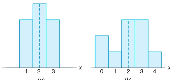
The mean, or expected value, of a random variable X is of special importance in statistics because it describes where the probability distribution is centered. By itself, however, the mean does not give an adequate description of the shape of the distribution. We also need to characterize the variability in the distribution. In Figure 4.1, we have the histograms of two discrete probability distributions that have the same mean,µ= 2, but differ considerably in variability, or the dispersion of their observations about the mean.

1 2 3 x 0 1 2 3 4

(a) (b)

x

Figure 4.1: Distributions with equal means and unequal dispersions.

The most important measure of variability of a random variableX is obtained by applying Theorem 4.1 with g(X) = (X−µ)2_{. The quantity is referred to as}

(11)

distribution of X and is denoted by Var(X) or the symbolσ2

X, or simply byσ

2

when it is clear to which random variable we refer.

Definition 4.3: _Let_X _{be a random variable with probability distribution}_f₍_x_{) and mean}_µ_{. The}

variance ofX is

σ2=E[(X−µ)2] =

x

(x−µ)2f(x), ifX is discrete, and

σ2=E[(X−µ)2] = ∞

−∞

(x−µ)2f(x)dx, ifX is continuous.

The positive square root of the variance,σ, is called thestandard deviationof

X.

The quantityx−µin Definition 4.3 is called thedeviation of an observation

from its mean. Since the deviations are squared and then averaged,σ2_{will be much}

smaller for a set of xvalues that are close to µthan it will be for a set of values that vary considerably fromµ.

Example 4.8: Let the random variableX represent the number of automobiles that are used for official business purposes on any given workday. The probability distribution for company A[Figure 4.1(a)] is

x 1 2 3

f(x) 0.3 0.4 0.3

and that for company B [Figure 4.1(b)] is

x 0 1 2 3 4

f(x) 0.2 0.1 0.3 0.3 0.1

Show that the variance of the probability distribution for company B is greater than that for company A.

Solution:For companyA, we find that

µA=E(X) = (1)(0.3) + (2)(0.4) + (3)(0.3) = 2.0,

and then

σ2_A=

3

x=1

(x−2)2= (1−2)2(0.3) + (2−2)2(0.4) + (3−2)2(0.3) = 0.6.

For companyB, we have

µB =E(X) = (0)(0.2) + (1)(0.1) + (2)(0.3) + (3)(0.3) + (4)(0.1) = 2.0,

and then

σ2

B=

4

x=0

(x−2)2_f₍_x₎

(12)

Clearly, the variance of the number of automobiles that are used for official business purposes is greater for companyB than for companyA.

An alternative and preferred formula for findingσ2_{, which often simplifies the}

calculations, is stated in the following theorem.

Theorem 4.2: The variance of a random variableX is

σ2=E(X2)−µ2.

Proof:For the discrete case, we can write

σ2=

x

(x−µ)2f(x) =

x

(x2−2µx+µ2)f(x)

=

x

x2f(x)−2µ

x

xf(x) +µ2

x

f(x).

Since µ =

x

xf(x) by definition, and

x

f(x) = 1 for any discrete probability

distribution, it follows that

σ2=

x

x2f(x)−µ2=E(X2)−µ2.

For the continuous case the proof is step by step the same, with summations replaced by integrations.

Example 4.9: Let the random variableX represent the number of defective parts for a machine when 3 parts are sampled from a production line and tested. The following is the probability distribution ofX.

x 0 1 2 3

f(x) 0.51 0.38 0.10 0.01 Using Theorem 4.2, calculateσ2_.

Solution:First, we compute

µ= (0)(0.51) + (1)(0.38) + (2)(0.10) + (3)(0.01) = 0.61.

Now,

E(X2) = (0)(0.51) + (1)(0.38) + (4)(0.10) + (9)(0.01) = 0.87.

Therefore,

σ2= 0.87−(0.61)2= 0.4979.

Example 4.10: The weekly demand for a drinking-water product, in thousands of liters, from a local chain of efficiency stores is a continuous random variable X having the probability density

f(x) =

2(x−1), 1< x <2,

0, elsewhere.

(13)

Solution:CalculatingE(X) andE(X2_{, we have}

µ=E(X) = 2 2

1

x(x−1)dx= 5 3

and

E(X2) = 2 2

1

x2(x−1)dx=17 6 .

Therefore,

σ2= 17 6 −

₅

3 2

= 1 18.

At this point, the variance or standard deviation has meaning only when we compare two or more distributions that have the same units of measurement. Therefore, we could compare the variances of the distributions of contents, mea-sured in liters, of bottles of orange juice from two companies, and the larger value would indicate the company whose product was more variable or less uniform. It would not be meaningful to compare the variance of a distribution of heights to the variance of a distribution of aptitude scores. In Section 4.4, we show how the standard deviation can be used to describe a single distribution of observations.

We shall now extend our concept of the variance of a random variable X to include random variables related toX. For the random variableg(X), the variance is denoted by σ2

g(X)and is calculated by means of the following theorem.

Theorem 4.3: LetX be a random variable with probability distributionf(x). The variance of the random variableg(X) is

σ2

g(X)=E{[g(X)−µg(X)]2}=

x

[g(x)−µg(X)]2f(x)

σ2

g(X)=E{[g(X)−µg(X)]2}=

∞

−∞

[g(x)−µg(X)]2f(x)dx

ifX is continuous.

Proof:Sinceg(X) is itself a random variable with meanµg(X)as defined in Theorem 4.1,

it follows from Definition 4.3 that

σ2

g(X)=E{[g(X)−µg(X)]}.

Now, applying Theorem 4.1 again to the random variable [g(X)−µg(X)]2completes

the proof.

Example 4.11: Calculate the variance of g(X) = 2X + 3, where X is a random variable with probability distribution

x 0 1 2 3

(14)

Solution:First, we find the mean of the random variable 2X+ 3. According to Theorem 4.1,

µ2X+3=E(2X+ 3) = 3

x=0

(2x+ 3)f(x) = 6.

Now, using Theorem 4.3, we have

σ2

2X+3=E{[(2X+ 3)−µ2x+3]2}=E[(2X+ 3−6)2]

=E(4X2−12X+ 9) =

3

x=0

(4x2−12x+ 9)f(x) = 4.

Example 4.12: LetX be a random variable having the density function given in Example 4.5 on page 115. Find the variance of the random variableg(X) = 4X+ 3.

Solution:In Example 4.5, we found thatµ4X+3= 8. Now, using Theorem 4.3, σ42X+3=E{[(4X+ 3)−8]2}=E[(4X−5)2]

= 2

−1

(4x−5)2x

2

3 dx= 1 3

2

−1

(16x4−40x3+ 25x2)dx= 51 5 .

Ifg(X, Y) = (X−µX)(Y−µY), whereµX =E(X) andµY =E(Y), Definition

4.2 yields an expected value called thecovariance ofX andY, which we denote byσX Y or Cov(X, Y).

Definition 4.4: _Let_X_and_Y _{be random variables with joint probability distribution}_f₍_{x, y}_{). The}

covariance ofX andY is

σX Y =E[(X−µX)(Y −µY)] =

x

y

(x−µX)(y−µy)f(x, y)

ifX andY are discrete, and

σX Y =E[(X−µX)(Y −µY)] = ∞

−∞ ∞

−∞

(x−µX)(y−µy)f(x, y)dx dy

ifX andY are continuous.

The covariance between two random variables is a measure of the nature of the association between the two. If large values ofX often result in large values ofY

(15)

The alternative and preferred formula forσX Y is stated by Theorem 4.4.

Theorem 4.4: The covariance of two random variablesX andY with meansµX andµY, respec-tively, is given by

σX Y =E(XY)−µXµY.

Proof:For the discrete case, we can write

σX Y =

for any joint discrete distribution, it follows that

σX Y =E(XY)−µXµY −µYµX+µXµY =E(XY)−µXµY.

For the continuous case, the proof is identical with summations replaced by inte-grals.

Example 4.13: Example 3.14 on page 95 describes a situation involving the number of blue refills

X and the number of red refills Y. Two refills for a ballpoint pen are selected at random from a certain box, and the following is the joint probability distribution:

x

Find the covariance ofX andY.

(16)

Therefore,

σX Y =E(XY)−µXµY = 3 14−

₃

4 1 2

=−₅₆9 .

Example 4.14: The fractionX of male runners and the fractionY of female runners who compete in marathon races are described by the joint density function

f(x, y) =

8xy, 0≤y≤x≤1,

0, elsewhere.

Find the covariance ofX andY.

Solution:We first compute the marginal density functions. They are

g(x) =

4x3_, ₀_≤_x_≤₁_,

0, elsewhere,

and

h(y) =

4y(1−y2), 0≤y≤1,

0, elsewhere.

From these marginal density functions, we compute

µX=E(X) = 1

0

4x4 dx= 4

5 andµY = 1

0

4y2(1−y2)dy= 8 15.

From the joint density function given above, we have

E(XY) = 1

0

1

y

8x2_y2_{dx dy}₌ 4

9.

Then

σX Y =E(XY)−µXµY = 4 9−

₄

5 8 15

= 4

225.

Although the covariance between two random variables does provide informa-tion regarding the nature of the relainforma-tionship, the magnitude ofσX Y does not

indi-cate anything regarding the strength of the relationship, sinceσX Y is not scale-free. Its magnitude will depend on the units used to measure bothX andY. There is a scale-free version of the covariance called thecorrelation coefficientthat is used widely in statistics.

Definition 4.5: _Let_X _and _Y _{be random variables with covariance}_σX Y and standard deviations

σX andσY, respectively. The correlation coefficient ofX andY is

ρX Y =

σX Y

σXσY

.

(17)

ρX Y = 1 if b > 0 and ρX Y =−1 if b < 0. (See Exercise 4.48.) The correlation coefficient is the subject of more discussion in Chapter 12, where we deal with linear regression.

Example 4.15: Find the correlation coefficient betweenX and Y in Example 4.13.

Solution:Since

Therefore, the correlation coefficient betweenX andY is

ρXY =

Example 4.16: Find the correlation coefficient ofX andY in Example 4.14.

Solution:Because

(18)

/ /

Exercises 127

Exercises

4.33 Use Deﬁnition 4.3 on page 120 to ﬁnd the vari-ance of the random variableXof Exercise 4.7 on page 117.

x −2 3 5

f(x) 0.3 0.2 0.5 Find the standard deviation ofX.

4.35 The random variableX, representing the num-ber of errors per 100 lines of software code, has the following probability distribution:

x 2 3 4 5 6

f(x) 0.01 0.25 0.4 0.3 0.04 Using Theorem 4.2 on page 121, ﬁnd the variance of

X.

4.36 Suppose that the probabilities are 0.4, 0.3, 0.2, and 0.1, respectively, that 0, 1, 2, or 3 power failures will strike a certain subdivision in any given year. Find the mean and variance of the random variableX repre-senting the number of power failures striking this sub-division.

4.37 A dealer’s proﬁt, in units of $5000, on a new automobile is a random variableX having the density function given in Exercise 4.12 on page 117. Find the variance ofX.

4.38 The proportion of people who respond to a cer-tain mail-order solicitation is a random variableX hav-ing the density function given in Exercise 4.14 on page 117. Find the variance ofX.

4.39 The total number of hours, in units of 100 hours, that a family runs a vacuum cleaner over a period of one year is a random variable X having the density function given in Exercise 4.13 on page 117. Find the variance ofX.

4.40 Referring to Exercise 4.14 on page 117, ﬁnd

σ2

g(X) for the functiong(X) = 3X2+ 4.

4.41 Find the standard deviation of the random vari-ableg(X) = (2X+ 1)2 in Exercise 4.17 on page 118.

4.42 Using the results of Exercise 4.21 on page 118, ﬁnd the variance ofg(X) =X2_{, where}_X _{is a random}

variable having the density function given in Exercise 4.12 on page 117.

4.43 The length of time, in minutes, for an airplane to obtain clearance for takeoﬀ at a certain airport is a

random variableY = 3X−2, whereXhas the density

Find the mean and variance of the random variableY.

4.44 Find the covariance of the random variablesX

andY of Exercise 3.39 on page 105.

4.47 For the random variablesX andY whose joint density function is given in Exercise 3.40 on page 105, ﬁnd the covariance.

4.48 Given a random variableX, with standard de-viationσX, and a random variableY =a+bX, show

that ifb <0, the correlation coeﬃcientρX Y =−1, and

ifb >0,ρX Y = 1.

4.49 Consider the situation in Exercise 4.32 on page 119. The distribution of the number of imperfections per 10 meters of synthetic failure is given by

x 0 1 2 3 4

f(x) 0.41 0.37 0.16 0.05 0.01 Find the variance and standard deviation of the num-ber of imperfections.

4.50 For a laboratory assignment, if the equipment is working, the density function of the observed outcome

X is

f(x) =

2(1−x), 0< x <1,

0, otherwise.

Find the variance and standard deviation ofX.

4.51 For the random variables X and Y in Exercise 3.39 on page 105, determine the correlation coeﬃcient betweenX andY.

4.52 Random variablesXandY follow a joint distri-bution

f(x, y) =

2, 0< x≤y <1,

0, otherwise.

Determine the correlation coeﬃcient between X and

(19)

4.3 Means and Variances of Linear Combinations of

Random Variables

We now develop some useful properties that will simplify the calculations of means and variances of random variables that appear in later chapters. These properties will permit us to deal with expectations in terms of other parameters that are either known or easily computed. All the results that we present here are valid for both discrete and continuous random variables. Proofs are given only for the continuous case. We begin with a theorem and two corollaries that should be, intuitively, reasonable to the reader.

Theorem 4.5: Ifaandb are constants, then

E(aX+b) =aE(X) +b.

Proof:By the definition of expected value,

E(aX+b) = ∞

−∞

(ax+b)f(x)dx=a

∞

−∞

xf(x)dx+b

∞

−∞

f(x)dx.

The first integral on the right isE(X) and the second integral equals 1. Therefore, we have

E(aX+b) =aE(X) +b.

Corollary 4.1: Settinga= 0, we see thatE(b) =b.

Corollary 4.2: Settingb= 0, we see thatE(aX) =aE(X).

Example 4.17: Applying Theorem 4.5 to the discrete random variable f(X) = 2X −1, rework Example 4.4 on page 115.

Solution:According to Theorem 4.5, we can write

E(2X−1) = 2E(X)−1.

Now

µ=E(X) =

9

x=4 xf(x)

= (4)

1 12

+ (5)

1 12

+ (6)

1 4

+ (7)

1 4

+ (8)

1 6

+ (9)

1 6

= 41

6 .

Therefore,

µ2X−1= (2)

41

6

−1 = $12.67,

(20)

4.3 Means and Variances of Linear Combinations of Random Variables 129

Example 4.18: Applying Theorem 4.5 to the continuous random variableg(X) = 4X+ 3, rework Example 4.5 on page 115.

Solution:For Example 4.5, we may use Theorem 4.5 to write

E(4X+ 3) = 4E(X) + 3.

Now

E(X) = 2

−1 x

_x2

3

dx= 2

−1 x3

3 dx= 5 4.

Therefore,

E(4X+ 3) = (4)

5 4

+ 3 = 8,

as before.

Theorem 4.6: The expected value of the sum or difference of two or more functions of a random variable X is the sum or difference of the expected values of the functions. That is,

E[g(X)±h(X)] =E[g(X)]±E[h(X)].

Proof:By definition,

E[g(X)±h(X)] = ∞

−∞

[g(x)±h(x)]f(x)dx

= ∞

−∞

g(x)f(x)dx± ∞

−∞

h(x)f(x)dx

=E[g(X)]±E[h(X)].

Example 4.19: LetX be a random variable with probability distribution as follows:

x 0 1 2 3

f(x) 1 3

1 2 0

1 6

Find the expected value ofY = (X−1)2_.

Solution:Applying Theorem 4.6 to the functionY = (X−1)2_{, we can write} E[(X−1)2] =E(X2−2X+ 1) =E(X2)−2E(X) +E(1).

From Corollary 4.1,E(1) = 1, and by direct computation,

E(X) = (0) ₁

3

+ (1) ₁

2

+ (2)(0) + (3) ₁

6

= 1 and

E(X2) = (0) ₁

3

+ (1) ₁

2

+ (4)(0) + (9) ₁

6

= 2.

Hence,

(21)

Example 4.20: The weekly demand for a certain drink, in thousands of liters, at a chain of con-venience stores is a continuous random variableg(X) =X2₊_X₋_{2, where}_X _has

the density function

f(x) =

2(x−1), 1< x <2,

0, elsewhere.

Find the expected value of the weekly demand for the drink.

Solution:By Theorem 4.6, we write

E(X2+X−2) =E(X2) +E(X)−E(2).

From Corollary 4.1,E(2) = 2, and by direct integration,

E(X) = 2

1

2x(x−1)dx= 5

3 andE(X

2_{) =} 2

1

2x2(x−1)dx= 17 6 .

Now

E(X2+X−2) = 17 6 +

5 3−2 =

5 2,

so the average weekly demand for the drink from this chain of efficiency stores is 2500 liters.

Suppose that we have two random variablesX andY with joint probability dis-tribution f(x, y). Two additional properties that will be very useful in succeeding chapters involve the expected values of the sum, difference, and product of these two random variables. First, however, let us prove a theorem on the expected value of the sum or difference of functions of the given variables. This, of course, is merely an extension of Theorem 4.6.

Theorem 4.7: The expected value of the sum or difference of two or more functions of the random variablesX andY is the sum or difference of the expected values of the functions. That is,

E[g(X, Y)±h(X, Y)] =E[g(X, Y)]±E[h(X, Y)].

Proof:By Definition 4.2,

E[g(X, Y)±h(X, Y)] = ∞

−∞ ∞

−∞

[g(x, y)±h(x, y)]f(x, y)dx dy

= ∞

−∞ ∞

−∞

g(x, y)f(x, y)dx dy± ∞

−∞ ∞

−∞

h(x, y)f(x, y)dx dy

=E[g(X, Y)]±E[h(X, Y)].

Corollary 4.3: Settingg(X, Y) =g(X) andh(X, Y) =h(Y), we see that

(22)

Corollary 4.4: Settingg(X, Y) =X andh(X, Y) =Y, we see that

E[X±Y] =E[X]±E[Y].

IfX represents the daily production of some item from machineAand Y the daily production of the same kind of item from machineB, thenX+Y represents the total number of items produced daily by both machines. Corollary 4.4 states that the average daily production for both machines is equal to the sum of the average daily production of each machine.

Theorem 4.8: LetX andY be two independent random variables. Then

E(XY) =E(X)E(Y).

Proof:By Definition 4.2,

E(XY) = ∞

−∞ ∞

−∞

xyf(x, y)dx dy.

SinceX andY are independent, we may write

f(x, y) =g(x)h(y),

whereg(x) andh(y) are the marginal distributions ofXandY, respectively. Hence,

E(XY) = ∞

−∞ ∞

−∞

xyg(x)h(y)dx dy= ∞

−∞

xg(x)dx

∞

−∞

yh(y)dy

=E(X)E(Y).

Theorem 4.8 can be illustrated for discrete variables by considering the exper-iment of tossing a green die and a red die. Let the random variable X represent the outcome on the green die and the random variable Y represent the outcome on the red die. ThenXY represents the product of the numbers that occur on the pair of dice. In the long run, the average of the products of the numbers is equal to the product of the average number that occurs on the green die and the average number that occurs on the red die.

Corollary 4.5: LetX andY be two independent random variables. ThenσX Y = 0.

Proof:The proof can be carried out by using Theorems 4.4 and 4.8.

Example 4.21: It is known that the ratio of gallium to arsenide does not affect the functioning of gallium-arsenide wafers, which are the main components of microchips. LetX

denote the ratio of gallium to arsenide andY denote the functional wafers retrieved during a 1-hour period. X andY are independent random variables with the joint density function

f(x, y) =

x(1+3y2 )

4 , 0< x <2, 0< y <1,

(23)

Show thatE(XY) =E(X)E(Y), as Theorem 4.8 suggests.

Solution:By definition,

E(XY) = 1

0

2

0

x2_y_{(1 + 3}_y2₎

4 dxdy= 5

6, E(X) = 4

3, andE(Y) = 5 8.

Hence,

E(X)E(Y) = ₄

3 5 8

= 5

6 =E(XY).

We conclude this section by proving one theorem and presenting several corol-laries that are useful for calculating variances or standard deviations.

Theorem 4.9: IfX andY are random variables with joint probability distributionf(x, y) anda,

b, andc are constants, then

σaX2 +bY+c =a2σ2X+b

2_σ2

Y + 2abσX Y.

Proof:By definition,σ2

aX+bY+c=E{[(aX+bY +c)−µaX+bY+c]2}. Now

µaX+bY+c =E(aX+bY +c) =aE(X) +bE(Y) +c=aµX+bµY +c,

by using Corollary 4.4 followed by Corollary 4.2. Therefore,

σ2_aX+bY+c=E{[a(X−µX) +b(Y −µY)]

2

} =a2E[(X−µX)

2_{] +}_b2_E_[(_Y

−µY)

2_{] + 2}_abE_[(_X

−µX)(Y −µY)] =a2σX2 +b

2_σ2

Y + 2abσX Y.

Using Theorem 4.9, we have the following corollaries.

Corollary 4.6: Settingb= 0, we see that

σ2aX+c=a2σX2 =a

2_σ2_.

Corollary 4.7: Settinga= 1 andb= 0, we see that

σX2+c=σ2X =σ

2_.

Corollary 4.8: Settingb= 0 andc= 0, we see that

σ2_aX =a2σ2X =a

2_σ2_.

(24)

Corollary 4.9: IfX andY are independent random variables, then

σaX2 +bY =a2σX2 +b

2_σ2

Y.

The result stated in Corollary 4.9 is obtained from Theorem 4.9 by invoking Corollary 4.5.

Corollary 4.10: IfX andY are independent random variables, then

σaX2 −bY =a2σX2 +b

2_σ2

Y.

Corollary 4.10 follows whenb in Corollary 4.9 is replaced by−b. Generalizing to a linear combination ofnindependent random variables, we have Corollary 4.11.

Corollary 4.11: IfX1, X2, . . . , Xn are independent random variables, then

σ2

a1X1+a2X2+···+anXn=a

2

1σX21+a 2

2σX22+· · ·+a 2

nσ2Xn.

Example 4.22: IfX andY are random variables with variancesσ2

X = 2 andσ

2

Y = 4 and covariance

σX Y =−2, find the variance of the random variableZ= 3X−4Y + 8.

Solution:

σ2Z=σ23X−4Y+8=σ23X−4Y (by Corollary 4.6)

= 9σX2 + 16σ

2

Y −24σX Y (by Theorem 4.9) = (9)(2) + (16)(4)−(24)(−2) = 130.

Example 4.23: Let X and Y denote the amounts of two different types of impurities in a batch of a certain chemical product. Suppose that X and Y are independent random variables with variances σ2

X = 2 and σ

2

Y = 3. Find the variance of the random variableZ = 3X−2Y + 5.

Solution:

σ2Z =σ23X−2Y+5=σ23X−2Y (by Corollary 4.6)

= 9σ2

x+ 4σy2 (by Corollary 4.10)

= (9)(2) + (4)(3) = 30.

What If the Function Is Nonlinear?

(25)

the expected value of linear combinations of random variables, there is no simple general rule. For example,

E(Z) =E(X/Y)= E(X)/E(Y),

except in very special circumstances.

The material provided by Theorems 4.5 through 4.9 and the various corollaries is extremely useful in that there are no restrictions on the form of the density or probability functions, apart from the property of independence when it is required as in the corollaries following Theorems 4.9. To illustrate, consider Example 4.23; the variance ofZ = 3X−2Y+5 does not require restrictions on the distributions of the amountsX andY of the two types of impurities. Only independence between

X and Y is required. Now, we do have at our disposal the capacity to findµg(X)

and σ2

g(X) for any functiong(·) from first principles established in Theorems 4.1

and 4.3, where it is assumed that the corresponding distribution f(x) is known. Exercises 4.40, 4.41, and 4.42, among others, illustrate the use of these theorems. Thus, if the function g(x) is nonlinear and the density function (or probability function in the discrete case) is known,µg(X) andσg2(X)can be evaluated exactly.

But, similar to the rules given for linear combinations, are there rules for nonlinear functions that can be used when the form of the distribution of the pertinent random variables is not known?

In general, supposeX is a random variable andY =g(x). The general solution for E(Y) or Var(Y) can be difficult to find and depends on the complexity of the functiong(·). However, there are approximations available that depend on a linear approximation of the function g(x). For example, suppose we denote E(X) asµ

and Var(X) = σ2_{X. Then a Taylor series approximation of} _g₍_x_{) around} _X ₌_µ

X gives

g(x) =g(µX) +

∂g(x)

∂x

x=µX

(x−µX) +

∂2_g₍_x₎ ∂x2

x=µX

(x−µX)

2

2 +· · · .

As a result, if we truncate after the linear term and take the expected value of both sides, we obtain E[g(X)] ≈g(µX), which is certainly intuitive and in some cases gives a reasonable approximation. However, if we include the second-order term of the Taylor series, then we have a second-order adjustment for this first-order approximation as follows:

Approximation of

E[g(X)] E[g(X)]≈g(µX) +

∂2_g₍_x₎ ∂x2

x=µX

σ2

X 2 .

Example 4.24: Given the random variableXwith meanµXand varianceσ2X, give the second-order approximation toE(eX_).

Solution:Since ∂ex

∂x =e

x _and ∂2 ex

∂x2 =ex, we obtainE(eX)≈eµ

X_{(1 +}_σ2 X/2).

Similarly, we can develop an approximation for Var[g(x)] by taking the variance of both sides of the first-order Taylor series expansion of g(x).

Approximation of

Var[g(X)] Var[g(X)]≈

_∂g₍_x₎

∂x

2

x=µX

σ2X.

(26)

4.4 Chebyshev’s Theorem 135

Solution:Again ∂ex

∂x =e

x_{; thus, Var(}_X₎_≈_e2µX_σ2 X.

These approximations can be extended to nonlinear functions of more than one random variable.

Given a set of independent random variables X1, X2, . . . , Xk with means µ1,

µ2, . . .,µk and variancesσ12, σ22, . . . , σk2, respectively, let

Y =h(X1, X2, . . . , Xk)

be a nonlinear function; then the following are approximations for E(Y) and Var(Y):

Example 4.26: Consider two independent random variablesX andZ with meansµX andµZ and variances σ2

X andσ

2

Z, respectively. Consider a random variable

Y =X/Z.

and the approximation for the variance ofY is given by

Var(Y)≈ _µ1₂

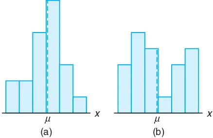
In Section 4.2 we stated that the variance of a random variable tells us something about the variability of the observations about the mean. If a random variable has a small variance or standard deviation, we would expect most of the values to be grouped around the mean. Therefore, the probability that the random variable assumes a value within a certain interval about the mean is greater than for a similar random variable with a larger standard deviation. If we think of probability in terms of area, we would expect a continuous distribution with a large value of

(27)

x µ

(a)

x µ

(b)

Figure 4.2: Variability of continuous observations about the mean.

µ x

(a)

µ x

(b)

Figure 4.3: Variability of discrete observations about the mean.

We can argue the same way for a discrete distribution. The area in the prob-ability histogram in Figure 4.3(b) is spread out much more than that in Figure 4.3(a) indicating a more variable distribution of measurements or outcomes.

The Russian mathematician P. L. Chebyshev (1821–1894) discovered that the fraction of the area between any two values symmetric about the mean is related to the standard deviation. Since the area under a probability distribution curve or in a probability histogram adds to 1, the area between any two numbers is the probability of the random variable assuming a value between these numbers.

(28)

/ /

Exercises 137

Theorem 4.10: (Chebyshev’s Theorem)The probability that any random variable X will as-sume a value withinkstandard deviations of the mean is at least 1−1/k2_{. That}

is,

P(µ−kσ < X < µ+kσ)≥1−_k12.

Fork= 2, the theorem states that the random variableX has a probability of at least 1−1/22= 3/4 of falling within two standard deviations of the mean. That is, three-fourths or more of the observations of any distribution lie in the interval

µ±2σ. Similarly, the theorem says that at least eight-ninths of the observations of any distribution fall in the intervalµ±3σ.

Example 4.27: A random variable X has a mean µ = 8, a variance σ2 _{= 9, and an unknown}

probability distribution. Find (a) P(−4< X <20), (b) P(|X−8| ≥6).

Solution: _(a) _P₍₋₄_{< X <}_{20) =}_P_[8₋₍₄₎₍₃₎_{< X <}_{8 + (4)(3)]}_≥ 15 16.

(b) P(|X−8| ≥6) = 1−P(|X−8|<6) = 1−P(−6< X−8<6)

= 1−P[8−(2)(3)< X <8 + (2)(3)]≤ 1₄.

Chebyshev’s theorem holds for any distribution of observations, and for this reason the results are usually weak. The value given by the theorem is a lower bound only. That is, we know that the probability of a random variable falling within two standard deviations of the mean can beno lessthan 3/4, but we never know how much more it might actually be. Only when the probability distribution is known can we determine exact probabilities. For this reason we call the theorem a distribution-free result. When specific distributions are assumed, as in future chapters, the results will be less conservative. The use of Chebyshev’s theorem is relegated to situations where the form of the distribution is unknown.

Exercises

4.53 Referring to Exercise 4.35 on page 127, ﬁnd the mean and variance of the discrete random variable

Z = 3X−2, whenX represents the number of errors per 100 lines of code.

4.54 Using Theorem 4.5 and Corollary 4.6, ﬁnd the mean and variance of the random variableZ= 5X+ 3, where X has the probability distribution of Exercise 4.36 on page 127.

4.55 Suppose that a grocery store purchases 5 car-tons of skim milk at the wholesale price of $1.20 per carton and retails the milk at $1.65 per carton. After the expiration date, the unsold milk is removed from the shelf and the grocer receives a credit from the

dis-tributor equal to three-fourths of the wholesale price. If the probability distribution of the random variable

X, the number of cartons that are sold from this lot, is

x 0 1 2 3 4 5

f(x) 1 15

2 15

3 15

4 15

3 15

ﬁnd the expected proﬁt.

4.56 Repeat Exercise 4.43 on page 127 by applying Theorem 4.5 and Corollary 4.6.

x −3 6 9

f(x) 1 6

1 2

(29)

/ /

Find E(X) and E(X2_{) and then, using these values,}

evaluateE[(2X+ 1)2_].

4.58 The total time, measured in units of 100 hours, that a teenager runs her hair dryer over a period of one year is a continuous random variable X that has the density function

Use Theorem 4.6 to evaluate the mean of the random variable Y = 60X2 _{+ 39}_X_{, where} _Y _{is equal to the}

number of kilowatt hours expended annually.

4.59 If a random variableX is deﬁned such that

E[(X−1)2] = 10 andE[(X−2)2] = 6,

ﬁndµandσ2_.

4.60 Suppose thatX andY are independent random variables having the joint probability distribution

x

for the joint probability distribution shown in Table 3.1 on page 96.

4.62 If X and Y are independent random variables with variances σ2

X = 5 andσ

2

Y = 3, ﬁnd the variance

of the random variableZ=−2X+ 4Y −3.

4.63 Repeat Exercise 4.62 if X andY are not inde-pendent andσX Y = 1.

4.64 Suppose thatX andY are independent random variables with probability densities and

g(x) =

4.65 LetXrepresent the number that occurs when a red die is tossed andY the number that occurs when a green die is tossed. Find

(a)E(X+Y); (b)E(X−Y);

(c)E(XY).

4.66 LetXrepresent the number that occurs when a green die is tossed andY the number that occurs when a red die is tossed. Find the variance of the random variable

(a) 2X−Y; (b)X+ 3Y −5.

4.67 If the joint density function ofX andY is given by

4.68 The power P in watts which is dissipated in an electric circuit with resistanceRis known to be given byP =I2_R_{, where}_I _{is current in amperes and}_R_{is a}

constant ﬁxed at 50 ohms. However,Iis a random vari-able withµI = 15 amperes and σ2I = 0.03 amperes2.

Give numerical approximations to the mean and vari-ance of the powerP.

4.69 Consider Review Exercise 3.77 on page 108. The random variablesXandY represent the number of ve-hicles that arrive at two separate street corners during a certain 2-minute period in the day. The joint distri-bution is

4.70 Consider Review Exercise 3.64 on page 107. There are two service lines. The random variables X

andY are the proportions of time that line 1 and line 2 are in use, respectively. The joint probability density function for (X, Y) is given by

(30)

/ /

Review Exercises 139

(b) It is of interest to know something about the pro-portion ofZ=X+Y, the sum of the two propor-tions. FindE(X+Y). Also ﬁndE(XY).

(c) Find Var(X), Var(Y), and Cov(X, Y). (d) Find Var(X+Y).

4.71 The length of time Y, in minutes, required to generate a human reﬂex to tear gas has the density function

(a) What is the mean time to reﬂex? (b) FindE(Y2_{) and Var(}_Y_).

4.72 A manufacturing company has developed a ma-chine for cleaning carpet that is fuel-eﬃcient because it delivers carpet cleaner so rapidly. Of interest is a random variableY, the amount in gallons per minute delivered. It is known that the density function is given by

f(y) =

1, 7≤y≤8,

0, elsewhere.

(a) Sketch the density function. (b) GiveE(Y),E(Y2_{), and Var(}_Y_).

4.73 For the situation in Exercise 4.72, compute

E(eY) using Theorem 4.1, that is, by using

using the second-order adjustment to the ﬁrst-order approximation ofE(eY_{). Comment.}

4.74 Consider again the situation of Exercise 4.72. It is required to ﬁnd Var(eY_{). Use Theorems 4.2 and 4.3}

and deﬁneZ=eY_{. Thus, use the conditions of}

Exer-cise 4.73 to ﬁnd

Var(Z) =E(Z2)−[E(Z)]2.

Then do it not by using f(y), but rather by using the ﬁrst-order Taylor series approximation to Var(eY). Comment!

4.75 An electrical ﬁrm manufactures a 100-watt light bulb, which, according to speciﬁcations written on the package, has a mean life of 900 hours with a standard deviation of 50 hours. At most, what percentage of the bulbs fail to last even 700 hours? Assume that the distribution is symmetric about the mean.

4.76 Seventy new jobs are opening up at an automo-bile manufacturing plant, and 1000 applicants show up for the 70 positions. To select the best 70 from among the applicants, the company gives a test that covers mechanical skill, manual dexterity, and mathematical ability. The mean grade on this test turns out to be 60, and the scores have a standard deviation of 6. Can a person who scores 84 count on getting one of the jobs? [Hint: Use Chebyshev’s theorem.] Assume that the distribution is symmetric about the mean.

4.77 A random variableX has a meanµ= 10 and a varianceσ2_{= 4. Using Chebyshev’s theorem, ﬁnd}

(a)P(|X−10| ≥3); (b)P(|X−10|<3); (c)P(5< X <15);

(d) the value of the constantcsuch that

P(|X−10| ≥c)≤0.04.

4.78 Compute P(µ−2σ < X < µ+ 2σ), whereX

has the density function

f(x) =

6x(1−x), 0< x <1,

0, elsewhere,

and compare with the result given in Chebyshev’s theorem.

Review Exercises

4.79 Prove Chebyshev’s theorem.

4.80 Find the covariance of random variablesX and

Y having the joint probability density function

f(x, y) =

x+y, 0< x <1, 0< y <1,

0, elsewhere.

4.81 Referring to the random variables whose joint probability density function is given in Exercise 3.47 on page 105, ﬁnd the average amount of kerosene left in the tank at the end of the day.

(31)

/ /

with probability density function

f(x) =

(b) Find the variance and standard deviation ofX. (c) FindE[(X+ 5)2_].

4.83 Referring to the random variables whose joint density function is given in Exercise 3.41 on page 105, ﬁnd the covariance between the weight of the creams and the weight of the toﬀees in these boxes of choco-lates.

4.84 Referring to the random variables whose joint probability density function is given in Exercise 3.41 on page 105, ﬁnd the expected weight for the sum of the creams and toﬀees if one purchased a box of these chocolates.

4.85 Suppose it is known that the lifeX of a partic-ular compressor, in hours, has the density function

f(x) =

1 900e−

x/900_, _{x >}₀_,

0, elsewhere.

(a) Find the mean life of the compressor. (b) FindE(X2_).

(c) Find the variance and standard deviation of the random variableX.

4.86 Referring to the random variables whose joint density function is given in Exercise 3.40 on page 105, (a) ﬁndµX andµY;

(b) ﬁndE[(X+Y)/2].

4.87 Show that Cov(aX, bY) =abCov(X, Y).

4.88 Consider the density function of Review Ex-ercise 4.85. Demonstrate that Chebyshev’s theorem holds fork= 2 andk= 3.

4.89 Consider the joint density function

f(x, y) =

16y

x3, x >2, 0< y <1,

0, elsewhere.

Compute the correlation coeﬃcientρX Y.

4.90 Consider random variablesXandY of Exercise 4.63 on page 138. ComputeρX Y.

4.91 A dealer’s proﬁt, in units of $5000, on a new au-tomobile is a random variableX having density func-tion

f(x) =

₂₍₁

−x), 0≤x≤1,

0, elsewhere.

(a) Find the variance of the dealer’s proﬁt.

(b) Demonstrate that Chebyshev’s theorem holds for

k= 2 with the density function above.

(c) What is the probability that the proﬁt exceeds $500?

4.92 Consider Exercise 4.10 on page 117. Can it be said that the ratings given by the two experts are in-dependent? Explain why or why not.

4.93 A company’s marketing and accounting depart-ments have determined that if the company markets its newly developed product, the contribution of the product to the ﬁrm’s proﬁt during the next 6 months will be described by the following:

Profit Contribution Probability What is the company’s expected proﬁt?

4.94 In a support system in the U.S. space program, a single crucial component works only 85% of the time. In order to enhance the reliability of the system, it is decided that 3 components will be installed in parallel such that the system fails only if they all fail. Assume the components act independently and that they are equivalent in the sense that all 3 of them have an 85% success rate. Consider the random variableX as the number of components out of 3 that fail.

(a) Write out a probability function for the random variableX.

(b) What is E(X) (i.e., the mean number of compo-nents out of 3 that fail)?

(c) What is Var(X)?

(d) What is the probability that the entire system is successful?

(e) What is the probability that the system fails? (f) If the desire is to have the system be successful

with probability 0.99, are three components suﬃ-cient? If not, how many are required?

(32)

/ /

(a) What is the expected proﬁt?

(b) Give the standard deviation of the proﬁt.

4.96 It is known through data collection and consid-erable research that the amount of time in seconds that a certain employee of a company is late for work is a random variableX with density function

f(x) =

In other words, he not only is slightly late at times, but also can be early to work.

(a) Find the expected value of the time in seconds that he is late.

(b) FindE(X2).

(c) What is the standard deviation of the amount of time he is late?

4.97 A delivery truck travels from pointAto pointB

and back using the same route each day. There are four traﬃc lights on the route. LetX1 denote the number

of red lights the truck encounters going from A toB

andX2 denote the number encountered on the return

trip. Data collected over a long period suggest that the joint probability distribution for (X1, X2) is given by

x2

(a) Give the marginal density ofX1.

(b) Give the marginal density ofX2.

(c) Give the conditional density distribution of X1

givenX2= 3.

(d) GiveE(X1).

(e) GiveE(X2).

(f) GiveE(X1 |X2 = 3).

(g) Give the standard deviation ofX1.

4.98 A convenience store has two separate locations where customers can be checked out as they leave. These locations each have two cash registers and two employees who check out customers. Let X be the number of cash registers being used at a particular time for location 1 andY the number being used at the same time for location 2. The joint probability function is given by

(a) Give the marginal density of bothXandY as well as the probability distribution ofX givenY = 2. (b) GiveE(X) and Var(X).

(c) GiveE(X |Y = 2) and Var(X |Y = 2).

4.99 Consider a ferry that can carry both buses and cars across a waterway. Each trip costs the owner ap-proximately $10. The fee for cars is $3 and the fee for buses is $8. LetX andY denote the number of buses and cars, respectively, carried on a given trip. The joint distribution ofX andY is given by

x

Compute the expected proﬁt for the ferry trip.

4.100 As we shall illustrate in Chapter 12, statistical methods associated with linear and nonlinear models are very important. In fact, exponential functions are often used in a wide variety of scientiﬁc and engineering problems. Consider a model that is ﬁt to a set of data involving measured valuesk1 andk2 and a certain

re-sponseY to the measurements. The model postulated is

of constants and hence are random variables. Assume that these random variables are independent and use the approximate formula for the variance of a nonlinear function of more than one variable. Give an expression for Var( ˆY). Assume that the means of b0, b1, and b2

are known and areβ0,β1, andβ2, and assume that the

variances ofb0, b1, and b2 are known and are σ20,σ12,

(33)

4.101 Consider Review Exercise 3.73 on page 108. It involved Y, the proportion of impurities in a batch, and the density function is given by

f(y) =

10(1−y)9, 0≤y≤1,

0, elsewhere.

(a) Find the expected percentage of impurities. (b) Find the expected value of the proportion of quality

material (i.e., ﬁndE(1−Y)).

(c) Find the variance of the random variableZ= 1−Y.

4.102 Project: LetX = number of hours each stu-dent in the class slept the night before. Create a dis-crete variable by using the following arbitrary intervals:

X <3, 3≤X <6, 6≤X <9, andX≥9. (a) Estimate the probability distribution forX. (b) Calculate the estimated mean and variance forX.

4.5 Potential Misconceptions and Hazards;

Relationship to Material in Other Chapters

The material in this chapter is extremely fundamental in nature, much like that in Chapter 3. Whereas in Chapter 3 we focused on general characteristics of a prob-ability distribution, in this chapter we defined important quantities orparameters

that characterize the general nature of the system. The mean of a distribution reflectscentral tendency, and thevarianceorstandard deviationreflects vari-abilityin the system. In addition, covariance reflects the tendency for two random variables to “move together” in a system. These important parameters will remain fundamental to all that follows in this text.