Probability & Statistics for
Engineers & Scientists
N I N T H
E D I T I O N
Ronald E. Walpole
Roanoke College
Raymond H. Myers
Virginia Tech
Sharon L. Myers
Radford University
Keying Ye
University of Texas at San Antonio
Chapter 5
Some Discrete Probability
Distributions
5.1
Introduction and Motivation
No matter whether a discrete probability distribution is represented graphically by a histogram, in tabular form, or by means of a formula, the behavior of a random variable is described. Often, the observations generated by different statistical ex-periments have the same general type of behavior. Consequently, discrete random variables associated with these experiments can be described by essentially the same probability distribution and therefore can be represented by a single formula. In fact, one needs only a handful of important probability distributions to describe many of the discrete random variables encountered in practice.
Such a handful of distributions describe several real-life random phenomena. For instance, in a study involving testing the effectiveness of a new drug, the num-ber of cured patients among all the patients who use the drug approximately follows a binomial distribution (Section 5.2). In an industrial example, when a sample of items selected from a batch of production is tested, the number of defective items in the sample usually can be modeled as a hypergeometric random variable (Sec-tion 5.3). In a statistical quality control problem, the experimenter will signal a shift of the process mean when observational data exceed certain limits. The num-ber of samples required to produce a false alarm follows a geometric distribution which is a special case of the negative binomial distribution (Section 5.4). On the other hand, the number of white cells from a fixed amount of an individual’s blood sample is usually random and may be described by a Poisson distribution (Section 5.5). In this chapter, we present these commonly used distributions with various examples.
5.2
Binomial and Multinomial Distributions
An experiment often consists of repeated trials, each with two possible outcomes that may be labeledsuccessorfailure. The most obvious application deals with
144 Chapter 5 Some Discrete Probability Distributions
the testing of items as they come off an assembly line, where each trial may indicate a defective or a nondefective item. We may choose to define either outcome as a success. The process is referred to as a Bernoulli process. Each trial is called a
Bernoulli trial. Observe, for example, if one were drawing cards from a deck, the probabilities for repeated trials change if the cards are not replaced. That is, the probability of selecting a heart on the first draw is 1/4, but on the second draw it is a conditional probability having a value of 13/51 or 12/51, depending on whether a heart appeared on the first draw: this, then, would no longer be considered a set of Bernoulli trials.
The Bernoulli Process
Strictly speaking, the Bernoulli process must possess the following properties: 1. The experiment consists of repeated trials.
2. Each trial results in an outcome that may be classified as a success or a failure. 3. The probability of success, denoted byp, remains constant from trial to trial. 4. The repeated trials are independent.
Consider the set of Bernoulli trials where three items are selected at random from a manufacturing process, inspected, and classified as defective or nondefective. A defective item is designated a success. The number of successes is a random variableXassuming integral values from 0 through 3. The eight possible outcomes and the corresponding values of X are
Outcome N N N N DN N N D DN N N DD DN D DDN DDD
x 0 1 1 1 2 2 2 3
Since the items are selected independently and we assume that the process produces 25% defectives, we have
P(N DN) =P(N)P(D)P(N) =
3 4
1 4
3 4
= 9 64.
Similar calculations yield the probabilities for the other possible outcomes. The probability distribution ofX is therefore
x 0 1 2 3
f(x) 27 64
27 64
9 64
1 64
Binomial Distribution
The number X of successes in n Bernoulli trials is called a binomial random variable. The probability distribution of this discrete random variable is called thebinomial distribution, and its values will be denoted byb(x;n, p) since they depend on the number of trials and the probability of a success on a given trial. Thus, for the probability distribution ofX, the number of defectives is
P(X = 2) =f(2) =b
2; 3,1
4
5.2 Binomial and Multinomial Distributions 145
Let us now generalize the above illustration to yield a formula for b(x;n, p). That is, we wish to find a formula that gives the probability of x successes in
n trials for a binomial experiment. First, consider the probability of xsuccesses and n−xfailures in a specified order. Since the trials are independent, we can multiply all the probabilities corresponding to the different outcomes. Each success occurs with probabilitypand each failure with probability q= 1−p. Therefore, the probability for the specified order ispxqn−x. We must now determine the total
number of sample points in the experiment that havexsuccesses andn−xfailures. This number is equal to the number of partitions of noutcomes into two groups withxin one group andn−xin the other and is writtenn
x
as introduced in Section 2.3. Because these partitions are mutually exclusive, we add the probabilities of all the different partitions to obtain the general formula, or simply multiply pxqn−x
bynx.
Binomial Distribution
A Bernoulli trial can result in a success with probability pand a failure with probabilityq= 1−p. Then the probability distribution of the binomial random variableX, the number of successes in nindependent trials, is
b(x;n, p) = of defectives, may be written as
b
rather than in the tabular form on page 144.
Example 5.1: The probability that a certain kind of component will survive a shock test is 3/4. Find the probability that exactly 2 of the next 4 components tested survive.
Solution:Assuming that the tests are independent and p= 3/4 for each of the 4 tests, we obtain
Where Does the Name
Binomial
Come From?
146 Chapter 5 Some Discrete Probability Distributions
a condition that must hold for any probability distribution.
Frequently, we are interested in problems where it is necessary to findP(X < r) or P(a≤X ≤b). Binomial sums
B(r;n, p) =
r
x=0
b(x;n, p)
are given in Table A.1 of the Appendix forn= 1,2, . . . ,20 for selected values ofp
from 0.1 to 0.9. We illustrate the use of Table A.1 with the following example.
Example 5.2: The probability that a patient recovers from a rare blood disease is 0.4. If 15 people are known to have contracted this disease, what is the probability that (a) at least 10 survive, (b) from 3 to 8 survive, and (c) exactly 5 survive?
Solution:LetX be the number of people who survive.
(a) P(X ≥10) = 1−P(X <10) = 1−
9
x=0
b(x; 15,0.4) = 1−0.9662 = 0.0338
(b) P(3≤X≤8) =
8
x=3
b(x; 15,0.4) =
8
x=0
b(x; 15,0.4)−
2
x=0
b(x; 15,0.4)
= 0.9050−0.0271 = 0.8779 (c) P(X= 5) =b(5; 15,0.4) =
5
x=0
b(x; 15,0.4)−
4
x=0
b(x; 15,0.4)
= 0.4032−0.2173 = 0.1859
Example 5.3: A large chain retailer purchases a certain kind of electronic device from a manu-facturer. The manufacturer indicates that the defective rate of the device is 3%.
(a) The inspector randomly picks 20 items from a shipment. What is the proba-bility that there will be at least one defective item among these 20?
(b) Suppose that the retailer receives 10 shipments in a month and the inspector randomly tests 20 devices per shipment. What is the probability that there will be exactly 3 shipments each containing at least one defective device among the 20 that are selected and tested from the shipment?
Solution: (a) Denote byX the number of defective devices among the 20. ThenX follows
a b(x; 20,0.03) distribution. Hence,
P(X≥1) = 1−P(X = 0) = 1−b(0; 20,0.03) = 1−(0.03)0
(1−0.03)20−0
= 0.4562.
(b) In this case, each shipment can either contain at least one defective item or not. Hence, testing of each shipment can be viewed as a Bernoulli trial with
5.2 Binomial and Multinomial Distributions 147
and denoting byY the number of shipments containing at least one defective item,Y follows another binomial distributionb(y; 10,0.4562). Therefore,
P(Y = 3) =
10
3
0.45623
(1−0.4562)7
= 0.1602.
Areas of Application
From Examples 5.1 through 5.3, it should be clear that the binomial distribution finds applications in many scientific fields. An industrial engineer is keenly inter-ested in the “proportion defective” in an industrial process. Often, quality control measures and sampling schemes for processes are based on the binomial distribu-tion. This distribution applies to any industrial situation where an outcome of a process is dichotomous and the results of the process are independent, with the probability of success being constant from trial to trial. The binomial distribution is also used extensively for medical and military applications. In both fields, a success or failure result is important. For example, “cure” or “no cure” is impor-tant in pharmaceutical work, and “hit” or “miss” is often the interpretation of the result of firing a guided missile.
Since the probability distribution of any binomial random variable depends only on the values assumed by the parameters n, p, andq, it would seem reasonable to assume that the mean and variance of a binomial random variable also depend on the values assumed by these parameters. Indeed, this is true, and in the proof of Theorem 5.1 we derive general formulas that can be used to compute the mean and variance of any binomial random variable as functions ofn,p, andq.
Theorem 5.1: The mean and variance of the binomial distributionb(x;n, p) are
µ=np andσ2
=npq.
Proof: Let the outcome on thejth trial be represented by a Bernoulli random variable
Ij, which assumes the values 0 and 1 with probabilities q and p, respectively.
Therefore, in a binomial experiment the number of successes can be written as the sum of the nindependent indicator variables. Hence,
X =I1+I2+· · ·+In.
The mean of anyIj isE(Ij) = (0)(q) + (1)(p) =p. Therefore, using Corollary 4.4
on page 131, the mean of the binomial distribution is
µ=E(X) =E(I1) +E(I2) +· · ·+E(In) =p+p+· · ·+p
n terms
=np.
The variance of anyIjisσI2j =E(I
2
j)−p
2
= (0)2
(q) + (1)2
(p)−p2
=p(1−p) =pq.
Extending Corollary 4.11 to the case ofnindependent Bernoulli variables gives the variance of the binomial distribution as
σ2
X=σ
2
I1+σ
2
I2+· · ·+σ
2
In=pq+pq+· · ·+pq
nterms
148 Chapter 5 Some Discrete Probability Distributions
Example 5.4: It is conjectured that an impurity exists in 30% of all drinking wells in a certain rural community. In order to gain some insight into the true extent of the problem, it is determined that some testing is necessary. It is too expensive to test all of the wells in the area, so 10 are randomly selected for testing.
(a) Using the binomial distribution, what is the probability that exactly 3 wells have the impurity, assuming that the conjecture is correct?
(b) What is the probability that more than 3 wells are impure?
Solution: (a) We require
b(3; 10,0.3) =
3
x=0
b(x; 10,0.3)−
2
x=0
b(x; 10,0.3) = 0.6496−0.3828 = 0.2668.
(b) In this case,P(X >3) = 1−0.6496 = 0.3504.
Example 5.5: Find the mean and variance of the binomial random variable of Example 5.2, and then use Chebyshev’s theorem (on page 137) to interpret the intervalµ±2σ.
Solution:Since Example 5.2 was a binomial experiment withn= 15 andp= 0.4, by Theorem 5.1, we have
µ= (15)(0.4) = 6 andσ2
= (15)(0.4)(0.6) = 3.6.
Taking the square root of 3.6, we find thatσ= 1.897. Hence, the required interval is 6±(2)(1.897), or from 2.206 to 9.794. Chebyshev’s theorem states that the number of recoveries among 15 patients who contracted the disease has a probability of at least 3/4 of falling between 2.206 and 9.794 or, because the data are discrete, between 2 and 10 inclusive.
There are solutions in which the computation of binomial probabilities may allow us to draw a scientific inference about population after data are collected. An illustration is given in the next example.
Example 5.6: Consider the situation of Example 5.4. The notion that 30% of the wells are impure is merely a conjecture put forth by the area water board. Suppose 10 wells are randomly selected and 6 are found to contain the impurity. What does this imply about the conjecture? Use a probability statement.
Solution:We must first ask: “If the conjecture is correct, is it likely that we would find 6 or more impure wells?”
P(X ≥6) =
10
x=0
b(x; 10,0.3)−
5
x=0
b(x; 10,0.3) = 1−0.9527 = 0.0473.
As a result, it is very unlikely (4.7% chance) that 6 or more wells would be found impure if only 30% of all are impure. This casts considerable doubt on the conjec-ture and suggests that the impurity problem is much more severe.
5.2 Binomial and Multinomial Distributions 149
Multinomial Experiments and the Multinomial Distribution
The binomial experiment becomes a multinomial experiment if we let each trial have more than two possible outcomes. The classification of a manufactured product as being light, heavy, or acceptable and the recording of accidents at a certain intersection according to the day of the week constitute multinomial exper-iments. The drawing of a card from a deckwith replacement is also a multinomial experiment if the 4 suits are the outcomes of interest.
In general, if a given trial can result in any one ofkpossible outcomesE1, E2, . . .,
Ek with probabilitiesp1, p2, . . . , pk, then themultinomial distribution will give
the probability that E1 occurs x1 times, E2 occurs x2 times, . . ., and Ek occurs
xk times innindependent trials, where
x1+x2+· · ·+xk =n.
We shall denote this joint probability distribution by
f(x1, x2, . . . , xk;p1, p2, . . . , pk, n).
Clearly,p1+p2+· · ·+pk = 1, since the result of each trial must be one of the k
possible outcomes.
To derive the general formula, we proceed as in the binomial case. Since the trials are independent, any specified order yielding x1 outcomes for E1, x2 for
E2, . . . , xk forEk will occur with probability px11p
x2
2 · · ·p
xk
k . The total number of
orders yielding similar outcomes for thentrials is equal to the number of partitions of n items into k groups with x1 in the first group, x2 in the second group, . . .,
andxk in thekth group. This can be done in
n x1, x2, . . . , xk
= n!
x1!x2!· · ·xk!
ways. Since all the partitions are mutually exclusive and occur with equal proba-bility, we obtain the multinomial distribution by multiplying the probability for a specified order by the total number of partitions.
Multinomial Distribution
If a given trial can result in thek outcomesE1, E2, . . . , Ek with probabilities
p1, p2, . . . , pk, then the probability distribution of the random variablesX1, X2,
. . . , Xk, representing the number of occurrences for E1, E2, . . . , Ek in n
inde-pendent trials, is
f(x1, x2, . . . , xk;p1, p2, . . . , pk, n) =
n x1, x2, . . . , xk
px1
1 p
x2
2 · · ·p
xk
k ,
with
k
i=1
xi=nand k
i=1
pi= 1.
The multinomial distribution derives its name from the fact that the terms of the multinomial expansion of (p1+p2+· · ·+pk)n correspond to all the possible
/ /
150 Chapter 5 Some Discrete Probability Distributions
Example 5.7: The complexity of arrivals and departures of planes at an airport is such that computer simulation is often used to model the “ideal” conditions. For a certain airport with three runways, it is known that in the ideal setting the following are the probabilities that the individual runways are accessed by a randomly arriving commercial jet:
Runway 1: p1= 2/9,
Runway 2: p2= 1/6,
Runway 3: p3= 11/18.
What is the probability that 6 randomly arriving airplanes are distributed in the following fashion?
Runway 1: 2 airplanes, Runway 2: 1 airplane, Runway 3: 3 airplanes
Solution:Using the multinomial distribution, we have
f
5.1 A random variable X that assumes the values
x1, x2, . . . , xkis called a discrete uniform random
vari-able if its probability mass function isf(x) = 1
k for all
of x1, x2, . . . , xk and 0 otherwise. Find the mean and
variance ofX.
5.2 Twelve people are given two identical speakers, which they are asked to listen to for differences, if any. Suppose that these people answer simply by guessing. Find the probability that three people claim to have heard a difference between the two speakers.
5.3 An employee is selected from a staff of 10 to super-vise a certain project by selecting a tag at random from a box containing 10 tags numbered from 1 to 10. Find the formula for the probability distribution ofX rep-resenting the number on the tag that is drawn. What is the probability that the number drawn is less than 4?
5.4 In a certain city district, the need for money to buy drugs is stated as the reason for 75% of all thefts. Find the probability that among the next 5 theft cases reported in this district,
(a) exactly 2 resulted from the need for money to buy drugs;
(b) at most 3 resulted from the need for money to buy drugs.
5.5 According to Chemical Engineering Progress
(November 1990), approximately 30% of all pipework failures in chemical plants are caused by operator error. (a) What is the probability that out of the next 20 pipework failures at least 10 are due to operator error?
(b) What is the probability that no more than 4 out of 20 such failures are due to operator error? (c) Suppose, for a particular plant, that out of the
ran-dom sample of 20 such failures, exactly 5 are due to operator error. Do you feel that the 30% figure stated above applies to this plant? Comment.
5.6 According to a survey by the Administrative Management Society, one-half of U.S. companies give employees 4 weeks of vacation after they have been with the company for 15 years. Find the probabil-ity that among 6 companies surveyed at random, the number that give employees 4 weeks of vacation after 15 years of employment is
(a) anywhere from 2 to 5; (b) fewer than 3.
5.7 One prominent physician claims that 70% of those with lung cancer are chain smokers. If his assertion is correct,
/ /
Exercises 151
recently admitted to a hospital, fewer than half are chain smokers;
(b) find the probability that of 20 such patients re-cently admitted to a hospital, fewer than half are chain smokers.
5.8 According to a study published by a group of Uni-versity of Massachusetts sociologists, approximately 60% of the Valium users in the state of Massachusetts first took Valium for psychological problems. Find the probability that among the next 8 users from this state who are interviewed,
(a) exactly 3 began taking Valium for psychological problems;
(b) at least 5 began taking Valium for problems that were not psychological.
5.9 In testing a certain kind of truck tire over rugged terrain, it is found that 25% of the trucks fail to com-plete the test run without a blowout. Of the next 15 trucks tested, find the probability that
(a) from 3 to 6 have blowouts; (b) fewer than 4 have blowouts; (c) more than 5 have blowouts.
5.10 A nationwide survey of college seniors by the University of Michigan revealed that almost 70% dis-approve of daily pot smoking, according to a report in
Parade. If 12 seniors are selected at random and asked their opinion, find the probability that the number who disapprove of smoking pot daily is
(a) anywhere from 7 to 9; (b) at most 5;
(c) not less than 8.
5.11 The probability that a patient recovers from a delicate heart operation is 0.9. What is the probabil-ity that exactly 5 of the next 7 patients having this operation survive?
5.12 A traffic control engineer reports that 75% of the vehicles passing through a checkpoint are from within the state. What is the probability that fewer than 4 of the next 9 vehicles are from out of state?
5.13 A national study that examined attitudes about antidepressants revealed that approximately 70% of re-spondents believe “antidepressants do not really cure anything, they just cover up the real trouble.” Accord-ing to this study, what is the probability that at least 3 of the next 5 people selected at random will hold this opinion?
5.14 The percentage of wins for the Chicago Bulls basketball team going into the playoffs for the 1996–97 season was 87.7. Round the 87.7 to 90 in order to use Table A.1.
(a) What is the probability that the Bulls sweep (4-0) the initial best-of-7 playoff series?
(b) What is the probability that the Bulls win the ini-tial best-of-7 playoff series?
(c) What very important assumption is made in an-swering parts (a) and (b)?
5.15 It is known that 60% of mice inoculated with a serum are protected from a certain disease. If 5 mice are inoculated, find the probability that
(a) none contracts the disease; (b) fewer than 2 contract the disease; (c) more than 3 contract the disease.
5.16 Suppose that airplane engines operate indepen-dently and fail with probability equal to 0.4. Assuming that a plane makes a safe flight if at least one-half of its engines run, determine whether a 4-engine plane or a 2-engine plane has the higher probability for a successful flight.
5.17 If X represents the number of people in Exer-cise 5.13 who believe that antidepressants do not cure but only cover up the real problem, find the mean and variance ofX when 5 people are selected at random.
5.18 (a) In Exercise 5.9, how many of the 15 trucks would you expect to have blowouts?
(b) What is the variance of the number of blowouts ex-perienced by the 15 trucks? What does that mean?
5.19 As a student drives to school, he encounters a traffic signal. This traffic signal stays green for 35 sec-onds, yellow for 5 secsec-onds, and red for 60 seconds. As-sume that the student goes to school each weekday between 8:00 and 8:30 a.m. LetX1 be the number of
times he encounters a green light, X2 be the number
of times he encounters a yellow light, andX3 be the
number of times he encounters a red light. Find the joint distribution ofX1,X2, andX3.
5.20 According toUSA Today(March 18, 1997), of 4 million workers in the general workforce, 5.8% tested positive for drugs. Of those testing positive, 22.5% were cocaine users and 54.4% marijuana users. (a) What is the probability that of 10 workers testing
positive, 2 are cocaine users, 5 are marijuana users, and 3 are users of other drugs?
152 Chapter 5 Some Discrete Probability Distributions
(c) What is the probability that of 10 workers testing positive, none is a cocaine user?
5.21 The surface of a circular dart board has a small center circle called the bull’s-eye and 20 pie-shaped re-gions numbered from 1 to 20. Each of the pie-shaped regions is further divided into three parts such that a person throwing a dart that lands in a specific region scores the value of the number, double the number, or triple the number, depending on which of the three parts the dart hits. If a person hits the bull’s-eye with probability 0.01, hits a double with probability 0.10, hits a triple with probability 0.05, and misses the dart board with probability 0.02, what is the probability that 7 throws will result in no bull’s-eyes, no triples, a double twice, and a complete miss once?
5.22 According to a genetics theory, a certain cross of guinea pigs will result in red, black, and white offspring in the ratio 8:4:4. Find the probability that among 8 offspring, 5 will be red, 2 black, and 1 white.
5.23 The probabilities are 0.4, 0.2, 0.3, and 0.1, re-spectively, that a delegate to a certain convention ar-rived by air, bus, automobile, or train. What is the probability that among 9 delegates randomly selected at this convention, 3 arrived by air, 3 arrived by bus, 1 arrived by automobile, and 2 arrived by train?
5.24 A safety engineer claims that only 40% of all workers wear safety helmets when they eat lunch at the workplace. Assuming that this claim is right, find the probability that 4 of 6 workers randomly chosen will be wearing their helmets while having lunch at the workplace.
5.25 Suppose that for a very large shipment of integrated-circuit chips, the probability of failure for any one chip is 0.10. Assuming that the assumptions underlying the binomial distributions are met, find the probability that at most 3 chips fail in a random sample of 20.
5.26 Assuming that 6 in 10 automobile accidents are due mainly to a speed violation, find the probabil-ity that among 8 automobile accidents, 6 will be due mainly to a speed violation
(a) by using the formula for the binomial distribution; (b) by using Table A.1.
5.27 If the probability that a fluorescent light has a useful life of at least 800 hours is 0.9, find the proba-bilities that among 20 such lights
(a) exactly 18 will have a useful life of at least 800 hours;
(b) at least 15 will have a useful life of at least 800 hours;
(c) at least 2 willnothave a useful life of at least 800 hours.
5.28 A manufacturer knows that on average 20% of the electric toasters produced require repairs within 1 year after they are sold. When 20 toasters are ran-domly selected, find appropriate numbersxandysuch that
(a) the probability that at leastxof them will require repairs is less than 0.5;
(b) the probability that at leastyof them willnot re-quire repairs is greater than 0.8.
5.3
Hypergeometric Distribution
The simplest way to view the distinction between the binomial distribution of Section 5.2 and the hypergeometric distribution is to note the way the sampling is done. The types of applications for the hypergeometric are very similar to those for the binomial distribution. We are interested in computing probabilities for the number of observations that fall into a particular category. But in the case of the binomial distribution, independence among trials is required. As a result, if that distribution is applied to, say, sampling from a lot of items (deck of cards, batch of production items), the sampling must be donewith replacementof each item after it is observed. On the other hand, the hypergeometric distribution does not require independence and is based on sampling done without replacement.
5.3 Hypergeometric Distribution 153
cards will serve as our first illustration.
If we wish to find the probability of observing 3 red cards in 5 draws from an ordinary deck of 52 playing cards, the binomial distribution of Section 5.2 does not apply unless each card is replaced and the deck reshuffled before the next draw is made. To solve the problem of sampling without replacement, let us restate the problem. If 5 cards are drawn at random, we are interested in the probability of selecting 3 red cards from the 26 available in the deck and 2 black cards from the 26 available in the deck. There are26
3
ways of selecting 3 red cards, and for each of these ways we can choose 2 black cards in26
2
ways. Therefore, the total number of ways to select 3 red and 2 black cards in 5 draws is the product 263
26 2
. The total number of ways to select any 5 cards from the 52 that are available is 525
. Hence, the probability of selecting 5 cards without replacement of which 3 are red and 2 are black is given by
26 3
26 2
52 5
=
(26!/3! 23!)(26!/2! 24!)
52!/5! 47! = 0.3251.
In general, we are interested in the probability of selecting x successes from the k items labeled successes and n−x failures from the N −k items labeled failures when a random sample of size nis selected fromN items. This is known as ahypergeometric experiment, that is, one that possesses the following two properties:
1. A random sample of sizenis selected without replacement fromN items. 2. Of the N items, kmay be classified as successes and N−kare classified as
failures.
The numberX of successes of a hypergeometric experiment is called a hyper-geometric random variable. Accordingly, the probability distribution of the hypergeometric variable is called the hypergeometric distribution, and its val-ues are denoted byh(x;N, n, k), since they depend on the number of successes k
in the set N from which we selectnitems.
Hypergeometric Distribution in Acceptance Sampling
Like the binomial distribution, the hypergeometric distribution finds applications in acceptance sampling, where lots of materials or parts are sampled in order to determine whether or not the entire lot is accepted.
Example 5.8: A particular part that is used as an injection device is sold in lots of 10. The producer deems a lot acceptable if no more than one defective is in the lot. A sampling plan involves random sampling and testing 3 of the parts out of 10. If none of the 3 is defective, the lot is accepted. Comment on the utility of this plan.
Solution:Let us assume that the lot is truly unacceptable(i.e., that 2 out of 10 parts are defective). The probability that the sampling plan finds the lot acceptable is
P(X = 0) =
2 0
8 3
10 3
154 Chapter 5 Some Discrete Probability Distributions
Thus, if the lot is truly unacceptable, with 2 defective parts, this sampling plan will allow acceptance roughly 47% of the time. As a result, this plan should be considered faulty.
Let us now generalize in order to find a formula for h(x;N, n, k). The total number of samples of size n chosen from N items is Nn. These samples are assumed to be equally likely. There are kxways of selectingxsuccesses from the
kthat are available, and for each of these ways we can choose then−xfailures in
N−k n−x
ways. Thus, the total number of favorable samples among theNnpossible samples is given bykxN−k
n−x
. Hence, we have the following definition.
Hypergeometric Distribution
The probability distribution of the hypergeometric random variableX, the num-ber of successes in a random sample of sizenselected fromN items of whichk
are labeledsuccessandN−klabeledfailure, is
h(x;N, n, k) =
k x
N−k n−x
N n
, max{0, n−(N−k)} ≤x≤min{n, k}.
The range of x can be determined by the three binomial coefficients in the definition, wherexandn−xare no more thankandN−k, respectively, and both of them cannot be less than 0. Usually, when both k (the number of successes) andN−k(the number of failures) are larger than the sample sizen, the range of a hypergeometric random variable will be x= 0,1, . . . , n.
Example 5.9: Lots of 40 components each are deemed unacceptable if they contain 3 or more defectives. The procedure for sampling a lot is to select 5 components at random and to reject the lot if a defective is found. What is the probability that exactly 1 defective is found in the sample if there are 3 defectives in the entire lot?
Solution:Using the hypergeometric distribution with n= 5,N = 40, k= 3, and x= 1, we find the probability of obtaining 1 defective to be
h(1; 40,5,3) =
3 1
37 4
40 5
= 0.3011.
Once again, this plan is not desirable since it detects a bad lot (3 defectives) only about 30% of the time.
Theorem 5.2: The mean and variance of the hypergeometric distributionh(x;N, n, k) are
µ= nk
N andσ
2
= N−n
N−1 ·n·
k N
1− k
N
.
The proof for the mean is shown in Appendix A.24.
5.3 Hypergeometric Distribution 155
Solution:Using the hypergeometric probability function, we have
h(3; 100,10,12) =
12 3
88 7
100 10
= 0.08.
Example 5.11: Find the mean and variance of the random variable of Example 5.9 and then use Chebyshev’s theorem to interpret the interval µ±2σ.
Solution: Since Example 5.9 was a hypergeometric experiment with N = 40, n = 5, and
k= 3, by Theorem 5.2, we have
µ=(5)(3) 40 =
3
8 = 0.375, and
σ2
=
40−5
39
(5)
3
40 1− 3 40
= 0.3113.
Taking the square root of 0.3113, we find that σ = 0.558. Hence, the required interval is 0.375 ± (2)(0.558), or from −0.741 to 1.491. Chebyshev’s theorem states that the number of defectives obtained when 5 components are selected at random from a lot of 40 components of which 3 are defective has a probability of at least 3/4 of falling between−0.741 and 1.491. That is, at least three-fourths of the time, the 5 components include fewer than 2 defectives.
Relationship to the Binomial Distribution
In this chapter, we discuss several important discrete distributions that have wide applicability. Many of these distributions relate nicely to each other. The beginning student should gain a clear understanding of these relationships. There is an interesting relationship between the hypergeometric and the binomial distribution. As one might expect, ifnis small compared toN, the nature of theNitems changes very little in each draw. So a binomial distribution can be used to approximate the hypergeometric distribution whennis small compared toN. In fact, as a rule of thumb, the approximation is good whenn/N≤0.05.
Thus, the quantity k/N plays the role of the binomial parameter p. As a result, the binomial distribution may be viewed as a large-population version of the hypergeometric distribution. The mean and variance then come from the formulas
µ=np=nk
N andσ
2
=npq=n· k
N
1− k
N
.
Comparing these formulas with those of Theorem 5.2, we see that the mean is the same but the variance differs by a correction factor of (N−n)/(N −1), which is negligible when nis small relative toN.
156 Chapter 5 Some Discrete Probability Distributions
Solution:SinceN= 5000 is large relative to the sample sizen= 10, we shall approximate the desired probability by using the binomial distribution. The probability of obtaining a blemished tire is 0.2. Therefore, the probability of obtaining exactly 3 blemished tires is
h(3; 5000,10,1000)≈b(3; 10,0.2) = 0.8791−0.6778 = 0.2013.
On the other hand, the exact probability ish(3; 5000,10,1000) = 0.2015.
The hypergeometric distribution can be extended to treat the case where the
N items can be partitioned intokcellsA1, A2, . . . , Ak witha1elements in the first
cell, a2 elements in the second cell,. . . , ak elements in the kth cell. We are now
interested in the probability that a random sample of size n yields x1 elements
from A1, x2 elements fromA2, . . . , and xk elements from Ak. Let us represent
this probability by
f(x1, x2, . . . , xk;a1, a2, . . . , ak, N, n).
To obtain a general formula, we note that the total number of samples of size
n that can be chosen fromN items is still Nn. There are a1
ways. Therefore, we can selectx1 items fromA1 and x2
items from A2 in
ways. Continuing in this way, we can select all nitems consisting of x1 fromA1,x2from A2,. . . ,andxk fromAk in
The required probability distribution is now defined as follows.
Multivariate Hypergeometric Distribution
IfN items can be partitioned into the kcellsA1, A2, . . . , Ak witha1, a2, . . . , ak
elements, respectively, then the probability distribution of the random vari-ables X1, X2, . . . , Xk, representing the number of elements selected from
Example 5.13: A group of 10 individuals is used for a biological case study. The group contains 3 people with blood type O, 4 with blood type A, and 3 with blood type B. What is the probability that a random sample of 5 will contain 1 person with blood type O, 2 people with blood type A, and 2 people with blood type B?
Solution:Using the extension of the hypergeometric distribution withx1= 1,x2= 2,x3= 2,
/ /
Exercises 157
Exercises
5.29 A homeowner plants 6 bulbs selected at ran-dom from a box containing 5 tulip bulbs and 4 daf-fodil bulbs. What is the probability that he planted 2 daffodil bulbs and 4 tulip bulbs?
5.30 To avoid detection at customs, a traveler places 6 narcotic tablets in a bottle containing 9 vitamin tablets that are similar in appearance. If the customs official selects 3 of the tablets at random for analysis, what is the probability that the traveler will be arrested for illegal possession of narcotics?
5.31 A random committee of size 3 is selected from 4 doctors and 2 nurses. Write a formula for the prob-ability distribution of the random variable X repre-senting the number of doctors on the committee. Find
P(2≤X≤3).
5.32 From a lot of 10 missiles, 4 are selected at ran-dom and fired. If the lot contains 3 defective missiles that will not fire, what is the probability that (a) all 4 will fire?
(b) at most 2 will not fire?
5.33 If 7 cards are dealt from an ordinary deck of 52 playing cards, what is the probability that
(a) exactly 2 of them will be face cards? (b) at least 1 of them will be a queen?
5.34 What is the probability that a waitress will refuse to serve alcoholic beverages to only 2 minors if she randomly checks the IDs of 5 among 9 students, 4 of whom are minors?
5.35 A company is interested in evaluating its cur-rent inspection procedure for shipments of 50 identical items. The procedure is to take a sample of 5 and pass the shipment if no more than 2 are found to be defective. What proportion of shipments with 20% de-fectives will be accepted?
5.36 A manufacturing company uses an acceptance scheme on items from a production line before they are shipped. The plan is a two-stage one. Boxes of 25 items are readied for shipment, and a sample of 3 items is tested for defectives. If any defectives are found, the entire box is sent back for 100% screening. If no defec-tives are found, the box is shipped.
(a) What is the probability that a box containing 3 defectives will be shipped?
(b) What is the probability that a box containing only 1 defective will be sent back for screening?
5.37 Suppose that the manufacturing company of Ex-ercise 5.36 decides to change its acceptance scheme. Under the new scheme, an inspector takes 1 item at random, inspects it, and then replaces it in the box; a second inspector does likewise. Finally, a third in-spector goes through the same procedure. The box is not shipped if any of the three inspectors find a de-fective. Answer the questions in Exercise 5.36 for this new plan.
5.38 Among 150 IRS employees in a large city, only 30 are women. If 10 of the employees are chosen at random to provide free tax assistance for the residents of this city, use the binomial approximation to the hy-pergeometric distribution to find the probability that at least 3 women are selected.
5.39 An annexation suit against a county subdivision of 1200 residences is being considered by a neighboring city. If the occupants of half the residences object to being annexed, what is the probability that in a ran-dom sample of 10 at least 3 favor the annexation suit?
5.40 It is estimated that 4000 of the 10,000 voting residents of a town are against a new sales tax. If 15 eligible voters are selected at random and asked their opinion, what is the probability that at most 7 favor the new tax?
5.41 A nationwide survey of 17,000 college seniors by the University of Michigan revealed that almost 70% disapprove of daily pot smoking. If 18 of these seniors are selected at random and asked their opinion, what is the probability that more than 9 but fewer than 14 disapprove of smoking pot daily?
5.42 Find the probability of being dealt a bridge hand of 13 cards containing 5 spades, 2 hearts, 3 diamonds, and 3 clubs.
5.43 A foreign student club lists as its members 2 Canadians, 3 Japanese, 5 Italians, and 2 Germans. If a committee of 4 is selected at random, find the prob-ability that
(a) all nationalities are represented;
(b) all nationalities except Italian are represented.
5.44 An urn contains 3 green balls, 2 blue balls, and 4 red balls. In a random sample of 5 balls, find the probability that both blue balls and at least 1 red ball are selected.
158 Chapter 5 Some Discrete Probability Distributions
the size of a population or the prevalence of certain features in the population. Ten animals of a certain population thought to be extinct (or near extinction) are caught, tagged, and released in a certain region. After a period of time, a random sample of 15 of this type of animal is selected in the region. What is the probability that 5 of those selected are tagged if there are 25 animals of this type in the region?
5.46 A large company has an inspection system for the batches of small compressors purchased from ven-dors. A batch typically contains 15 compressors. In the inspection system, a random sample of 5 is selected and all are tested. Suppose there are 2 faulty compressors in the batch of 15.
(a) What is the probability that for a given sample there will be 1 faulty compressor?
(b) What is the probability that inspection will dis-cover both faulty compressors?
5.47 A government task force suspects that some manufacturing companies are in violation of federal pollution regulations with regard to dumping a certain type of product. Twenty firms are under suspicion but not all can be inspected. Suppose that 3 of the firms are in violation.
(a) What is the probability that inspection of 5 firms will find no violations?
(b) What is the probability that the plan above will find two violations?
5.48 Every hour, 10,000 cans of soda are filled by a machine, among which 300 underfilled cans are pro-duced. Each hour, a sample of 30 cans is randomly selected and the number of ounces of soda per can is checked. Denote by X the number of cans selected that are underfilled. Find the probability that at least 1 underfilled can will be among those sampled.
5.4
Negative Binomial and Geometric Distributions
Let us consider an experiment where the properties are the same as those listed for a binomial experiment, with the exception that the trials will be repeated until a
fixednumber of successes occur. Therefore, instead of the probability ofxsuccesses in ntrials, wherenis fixed, we are now interested in the probability that thekth success occurs on the xth trial. Experiments of this kind are called negative binomial experiments.
As an illustration, consider the use of a drug that is known to be effective in 60% of the cases where it is used. The drug will be considered a success if it is effective in bringing some degree of relief to the patient. We are interested in finding the probability that the fifth patient to experience relief is the seventh patient to receive the drug during a given week. Designating a success byS and a failure by F, a possible order of achieving the desired result isSF SSSF S, which occurs with probability
(0.6)(0.4)(0.6)(0.6)(0.6)(0.4)(0.6) = (0.6)5
(0.4)2
.
We could list all possible orders by rearranging theF’s andS’s except for the last outcome, which must be the fifth success. The total number of possible orders is equal to the number of partitions of the first six trials into two groups with 2 failures assigned to the one group and 4 successes assigned to the other group. This can be done in 64
= 15 mutually exclusive ways. Hence, ifX represents the outcome on which the fifth success occurs, then
P(X = 7) =
6 4
(0.6)5
(0.4)2
= 0.1866.
What Is the Negative Binomial Random Variable?
5.4 Negative Binomial and Geometric Distributions 159
distribution is called thenegative binomial distribution. Since its probabilities depend on the number of successes desired and the probability of a success on a given trial, we shall denote them by b∗
(x;k, p). To obtain the general formula for b∗
(x;k, p), consider the probability of a success on the xth trial preceded by
k−1 successes and x−k failures in some specified order. Since the trials are independent, we can multiply all the probabilities corresponding to each desired outcome. Each success occurs with probabilitypand each failure with probability
q= 1−p. Therefore, the probability for the specified order ending in success is
pk−1
qx−kp=pkqx−k.
The total number of sample points in the experiment ending in a success, after the occurrence ofk−1 successes andx−kfailures in any order, is equal to the number of partitions ofx−1 trials into two groups withk−1 successes corresponding to one group andx−kfailures corresponding to the other group. This number is specified by the term x−1
k−1
, each mutually exclusive and occurring with equal probability
pkqx−k. We obtain the general formula by multiplyingpkqx−k byx−1
k−1
.
Negative Binomial Distribution
If repeated independent trials can result in a success with probability p and a failure with probability q = 1−p, then the probability distribution of the random variableX, the number of the trial on which the kth success occurs, is
b∗
(x;k, p) =
x−1 k−1
pkqx−k, x=k, k+ 1, k+ 2, . . . .
Example 5.14: In an NBA (National Basketball Association) championship series, the team that wins four games out of seven is the winner. Suppose that teamsAandB face each other in the championship games and that teamAhas probability 0.55 of winning a game over teamB.
(a) What is the probability that teamAwill win the series in 6 games? (b) What is the probability that teamAwill win the series?
(c) If teamsAandB were facing each other in a regional playoff series, which is decided by winning three out of five games, what is the probability that team
Awould win the series?
Solution: (a) b∗
(6; 4,0.55) =53
0.554
(1−0.55)6−4
= 0.1853 (b) P(teamAwins the championship series) is
b∗
(4; 4,0.55) +b∗
(5; 4,0.55) +b∗
(6; 4,0.55) +b∗
(7; 4,0.55) = 0.0915 + 0.1647 + 0.1853 + 0.1668 = 0.6083.
(c) P(teamAwins the playoff) is
b∗
(3; 3,0.55) +b∗
(4; 3,0.55) +b∗
160 Chapter 5 Some Discrete Probability Distributions
The negative binomial distribution derives its name from the fact that each term in the expansion of pk(1−q)−k corresponds to the values of b∗
(x;k, p) for
x=k, k+ 1, k+ 2, . . .. If we consider the special case of the negative binomial distribution where k = 1, we have a probability distribution for the number of trials required for a single success. An example would be the tossing of a coin until a head occurs. We might be interested in the probability that the first head occurs on the fourth toss. The negative binomial distribution reduces to the form
b∗
(x; 1, p) =pqx−1
, x= 1,2,3, . . . .
Since the successive terms constitute a geometric progression, it is customary to refer to this special case as thegeometric distribution and denote its values by
g(x;p).
Geometric Distribution
If repeated independent trials can result in a success with probability p and a failure with probability q = 1−p, then the probability distribution of the random variableX, the number of the trial on which the first success occurs, is
g(x;p) =pqx−1
, x= 1,2,3, . . . .
Example 5.15: For a certain manufacturing process, it is known that, on the average, 1 in every 100 items is defective. What is the probability that the fifth item inspected is the first defective item found?
Solution:Using the geometric distribution with x= 5 and p= 0.01, we have
g(5; 0.01) = (0.01)(0.99)4
= 0.0096.
Example 5.16: At a “busy time,” a telephone exchange is very near capacity, so callers have difficulty placing their calls. It may be of interest to know the number of attempts necessary in order to make a connection. Suppose that we let p = 0.05 be the probability of a connection during a busy time. We are interested in knowing the probability that 5 attempts are necessary for a successful call.
Solution:Using the geometric distribution with x= 5 and p= 0.05 yields
P(X =x) =g(5; 0.05) = (0.05)(0.95)4
= 0.041.
Quite often, in applications dealing with the geometric distribution, the mean and variance are important. For example, in Example 5.16, the expected number of calls necessary to make a connection is quite important. The following theorem states without proof the mean and variance of the geometric distribution.
Theorem 5.3: The mean and variance of a random variable following the geometric distribution are
µ= 1
p andσ
2
=1−p
5.5 Poisson Distribution and the Poisson Process 161
Applications of Negative Binomial and Geometric Distributions
Areas of application for the negative binomial and geometric distributions become obvious when one focuses on the examples in this section and the exercises devoted to these distributions at the end of Section 5.5. In the case of the geometric distribution, Example 5.16 depicts a situation where engineers or managers are attempting to determine how inefficient a telephone exchange system is during busy times. Clearly, in this case, trials occurring prior to a success represent a cost. If there is a high probability of several attempts being required prior to making a connection, then plans should be made to redesign the system.
Applications of the negative binomial distribution are similar in nature. Sup-pose attempts are costly in some sense and are occurring in sequence. A high probability of needing a “large” number of attempts to experience a fixed number of successes is not beneficial to the scientist or engineer. Consider the scenarios of Review Exercises 5.90 and 5.91. In Review Exercise 5.91, the oil driller defines a certain level of success from sequentially drilling locations for oil. If only 6 at-tempts have been made at the point where the second success is experienced, the profits appear to dominate substantially the investment incurred by the drilling.
5.5
Poisson Distribution and the Poisson Process
Experiments yielding numerical values of a random variable X, the number of outcomes occurring during a given time interval or in a specified region, are called
Poisson experiments. The given time interval may be of any length, such as a minute, a day, a week, a month, or even a year. For example, a Poisson experiment can generate observations for the random variable X representing the number of telephone calls received per hour by an office, the number of days school is closed due to snow during the winter, or the number of games postponed due to rain during a baseball season. The specified region could be a line segment, an area, a volume, or perhaps a piece of material. In such instances, X might represent the number of field mice per acre, the number of bacteria in a given culture, or the number of typing errors per page. A Poisson experiment is derived from the
Poisson processand possesses the following properties.
Properties of the Poisson Process
1. The number of outcomes occurring in one time interval or specified region of space is independent of the number that occur in any other disjoint time in-terval or region. In this sense we say that the Poisson process has no memory. 2. The probability that a single outcome will occur during a very short time interval or in a small region is proportional to the length of the time interval or the size of the region and does not depend on the number of outcomes occurring outside this time interval or region.
3. The probability that more than one outcome will occur in such a short time interval or fall in such a small region is negligible.
The numberX of outcomes occurring during a Poisson experiment is called a
162 Chapter 5 Some Discrete Probability Distributions
distribution. The mean number of outcomes is computed from µ = λt, where
t is the specific “time,” “distance,” “area,” or “volume” of interest. Since the probabilities depend on λ, the rate of occurrence of outcomes, we shall denote them by p(x;λt). The derivation of the formula for p(x;λt), based on the three properties of a Poisson process listed above, is beyond the scope of this book. The following formula is used for computing Poisson probabilities.
Poisson Distribution
The probability distribution of the Poisson random variable X, representing the number of outcomes occurring in a given time interval or specified region denoted byt, is
p(x;λt) = e
−λt(λt)x
x! , x= 0,1,2, . . . ,
where λ is the average number of outcomes per unit time, distance, area, or volume ande= 2.71828. . ..
Table A.2 contains Poisson probability sums,
P(r;λt) =
r
x=0
p(x;λt),
for selected values ofλtranging from 0.1 to 18.0. We illustrate the use of this table with the following two examples.
Example 5.17: During a laboratory experiment, the average number of radioactive particles pass-ing through a counter in 1 millisecond is 4. What is the probability that 6 particles enter the counter in a given millisecond?
Solution:Using the Poisson distribution with x= 6 andλt= 4 and referring to Table A.2, we have
p(6; 4) = e
−4
46
6! =
6
x=0
p(x; 4)−
5
x=0
p(x; 4) = 0.8893−0.7851 = 0.1042.
Example 5.18: Ten is the average number of oil tankers arriving each day at a certain port. The facilities at the port can handle at most 15 tankers per day. What is the probability that on a given day tankers have to be turned away?
Solution:LetX be the number of tankers arriving each day. Then, using Table A.2, we have
P(X >15) = 1−P(X ≤15) = 1−
15
x=0
p(x; 10) = 1−0.9513 = 0.0487.
Like the binomial distribution, the Poisson distribution is used for quality con-trol, quality assurance, and acceptance sampling. In addition, certain important continuous distributions used in reliability theory and queuing theory depend on the Poisson process. Some of these distributions are discussed and developed in Chapter 6. The following theorem concerning the Poisson random variable is given in Appendix A.25.
5.5 Poisson Distribution and the Poisson Process 163
Nature of the Poisson Probability Function
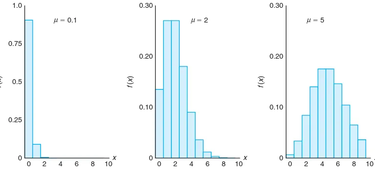
Like so many discrete and continuous distributions, the form of the Poisson distri-bution becomes more and more symmetric, even bell-shaped, as the mean grows large. Figure 5.1 illustrates this, showing plots of the probability function for
µ = 0.1, µ = 2, and µ = 5. Note the nearness to symmetry when µ becomes as large as 5. A similar condition exists for the binomial distribution, as will be illustrated later in the text.
0 0.25 0.5 0.75 1.0
0 2 4 6 8 10x
f
(
x
)
f
(
x
)
⫽ 0.1 ⫽ 2 ⫽ 5
0 0.10 0.20 0.30
f
(
x
)
0 0.10 0.20 0.30
x x
0 2 4 6 8 10 0 2 4 6 8 10
µ µ µ
Figure 5.1: Poisson density functions for different means.
Approximation of Binomial Distribution by a Poisson Distribution
It should be evident from the three principles of the Poisson process that the Poisson distribution is related to the binomial distribution. Although the Poisson usually finds applications in space and time problems, as illustrated by Examples 5.17 and 5.18, it can be viewed as a limiting form of the binomial distribution. In the case of the binomial, ifnis quite large andpis small, the conditions begin to simulate thecontinuous space or timeimplications of the Poisson process. The in-dependence among Bernoulli trials in the binomial case is consistent with principle 2 of the Poisson process. Allowing the parameterpto be close to 0 relates to prin-ciple 3 of the Poisson process. Indeed, ifnis large andpis close to 0, the Poisson distribution can be used, withµ =np, to approximate binomial probabilities. If
pis close to 1, we can still use the Poisson distribution to approximate binomial probabilities by interchanging what we have defined to be a success and a failure, thereby changingpto a value close to 0.
Theorem 5.5: LetXbe a binomial random variable with probability distributionb(x;n, p). When
n→ ∞, p→0, andnpn→∞
−→ µremains constant,
/ /
164 Chapter 5 Some Discrete Probability Distributions
Example 5.19: In a certain industrial facility, accidents occur infrequently. It is known that the probability of an accident on any given day is 0.005 and accidents are independent of each other.
(a) What is the probability that in any given period of 400 days there will be an accident on one day?
(b) What is the probability that there are at most three days with an accident?
Solution:LetX be a binomial random variable withn= 400 andp= 0.005. Thus, np= 2. Using the Poisson approximation,
(a) P(X = 1) =e−2
21
= 0.271 and
(b) P(X ≤3) =
3
x=0
e−2
2x/x! = 0.857.
Example 5.20: In a manufacturing process where glass products are made, defects or bubbles occur, occasionally rendering the piece undesirable for marketing. It is known that, on average, 1 in every 1000 of these items produced has one or more bubbles. What is the probability that a random sample of 8000 will yield fewer than 7 items possessing bubbles?
Solution: This is essentially a binomial experiment with n = 8000 and p = 0.001. Since
p is very close to 0 and n is quite large, we shall approximate with the Poisson distribution using
µ= (8000)(0.001) = 8.
Hence, if X represents the number of bubbles, we have
P(X <7) =
6
x=0
b(x; 8000,0.001)≈p(x; 8) = 0.3134.
Exercises
5.49 The probability that a person living in a certain city owns a dog is estimated to be 0.3. Find the prob-ability that the tenth person randomly interviewed in that city is the fifth one to own a dog.
5.50 Find the probability that a person flipping a coin gets
(a) the third head on the seventh flip; (b) the first head on the fourth flip.
5.51 Three people toss a fair coin and the odd one pays for coffee. If the coins all turn up the same, they are tossed again. Find the probability that fewer than 4 tosses are needed.
5.52 A scientist inoculates mice, one at a time, with a disease germ until he finds 2 that have contracted the
disease. If the probability of contracting the disease is 1/6, what is the probability that 8 mice are required?
5.53 An inventory study determines that, on aver-age, demands for a particular item at a warehouse are made 5 times per day. What is the probability that on a given day this item is requested
(a) more than 5 times? (b) not at all?
/ /
Exercises 165
(b) the third prescribing Valium for a woman.
5.55 The probability that a student pilot passes the written test for a private pilot’s license is 0.7. Find the probability that a given student will pass the test (a) on the third try;
(b) before the fourth try.
5.56 On average, 3 traffic accidents per month occur at a certain intersection. What is the probability that in any given month at this intersection
(a) exactly 5 accidents will occur? (b) fewer than 3 accidents will occur? (c) at least 2 accidents will occur?
5.57 On average, a textbook author makes two word-processing errors per page on the first draft of her text-book. What is the probability that on the next page she will make
(a) 4 or more errors? (b) no errors?
5.58 A certain area of the eastern United States is, on average, hit by 6 hurricanes a year. Find the prob-ability that in a given year that area will be hit by (a) fewer than 4 hurricanes;
(b) anywhere from 6 to 8 hurricanes.
5.59 Suppose the probability that any given person will believe a tale about the transgressions of a famous actress is 0.8. What is the probability that
(a) the sixth person to hear this tale is the fourth one to believe it?
(b) the third person to hear this tale is the first one to believe it?
5.60 The average number of field mice per acre in a 5-acre wheat field is estimated to be 12. Find the probability that fewer than 7 field mice are found (a) on a given acre;
(b) on 2 of the next 3 acres inspected.
5.61 Suppose that, on average, 1 person in 1000 makes a numerical error in preparing his or her income tax return. If 10,000 returns are selected at random and examined, find the probability that 6, 7, or 8 of them contain an error.
5.62 The probability that a student at a local high school fails the screening test for scoliosis (curvature of the spine) is known to be 0.004. Of the next 1875 students at the school who are screened for scoliosis,
find the probability that (a) fewer than 5 fail the test; (b) 8, 9, or 10 fail the test.
5.63 Find the mean and variance of the random vari-ableX in Exercise 5.58, representing the number of hurricanes per year to hit a certain area of the eastern United States.
5.64 Find the mean and variance of the random vari-ableX in Exercise 5.61, representing the number of persons among 10,000 who make an error in preparing their income tax returns.
5.65 An automobile manufacturer is concerned about a fault in the braking mechanism of a particular model. The fault can, on rare occasions, cause a catastrophe at high speed. The distribution of the number of cars per year that will experience the catastrophe is a Poisson random variable withλ= 5.
(a) What is the probability that at most 3 cars per year will experience a catastrophe?
(b) What is the probability that more than 1 car per year will experience a catastrophe?
5.66 Changes in airport procedures require consid-erable planning. Arrival rates of aircraft are impor-tant factors that must be taken into account. Suppose small aircraft arrive at a certain airport, according to a Poisson process, at the rate of 6 per hour. Thus, the Poisson parameter for arrivals over a period of hours is
µ= 6t.
(a) What is the probability that exactly 4 small air-craft arrive during a 1-hour period?
(b) What is the probability that at least 4 arrive during a 1-hour period?
(c) If we define a working day as 12 hours, what is the probability that at least 75 small aircraft ar-rive during a working day?
5.67 The number of customers arriving per hour at a certain automobile service facility is assumed to follow a Poisson distribution with meanλ= 7.
(a) Compute the probability that more than 10 cus-tomers will arrive in a 2-hour period.
(b) What is the mean number of arrivals during a 2-hour period?
5.68 Consider Exercise 5.62. What is the mean num-ber of students who fail the test?
/ /
166 Chapter 5 Some Discrete Probability Distributions
5.70 A company purchases large lots of a certain kind of electronic device. A method is used that rejects a lot if 2 or more defective units are found in a random sample of 100 units.
(a) What is the mean number of defective units found in a sample of 100 units if the lot is 1% defective? (b) What is the variance?
5.71 For a certain type of copper wire, it is known that, on the average, 1.5 flaws occur per millimeter. Assuming that the number of flaws is a Poisson random variable, what is the probability that no flaws occur in a certain portion of wire of length 5 millimeters? What is the mean number of flaws in a portion of length 5 millimeters?
5.72 Potholes on a highway can be a serious problem, and are in constant need of repair. With a particular type of terrain and make of concrete, past experience suggests that there are, on the average, 2 potholes per mile after a certain amount of usage. It is assumed that the Poisson process applies to the random vari-able “number of potholes.”
(a) What is the probability that no more than one pot-hole will appear in a section of 1 mile?
(b) What is the probability that no more than 4 pot-holes will occur in a given section of 5 miles?
5.73 Hospital administrators in large cities anguish about traffic in emergency rooms. At a particular hos-pital in a large city, the staff on hand cannot
accom-modate the patient traffic if there are more than 10 emergency cases in a given hour. It is assumed that patient arrival follows a Poisson process, and historical data suggest that, on the average, 5 emergencies arrive per hour.
(a) What is the probability that in a given hour the staff cannot accommodate the patient traffic? (b) What is the probability that more than 20
emer-gencies arrive during a 3-hour shift?
5.74 It is known that 3% of people whose luggage is screened at an airport have questionable objects in their luggage. What is the probability that a string of 15 people pass through screening successfully before an individual is caught with a questionable object? What is the expected number of people to pass through be-fore an individual is stopped?
5.75 Computer technology has produced an environ-ment in which robots operate with the use of micro-processors. The probability that a robot fails during any 6-hour shift is 0.10. What is the probability that a robot will operate through at most 5 shifts before it fails?
5.76 The refusal rate for telephone polls is known to be approximately 20%. A newspaper report indicates that 50 people were interviewed before the first refusal. (a) Comment on the validity of the report. Use a
prob-ability in your argument.
(b) What is the expected number of people interviewed before a refusal?
Review Exercises
5.77 During a manufacturing process, 15 units are randomly selected each day from the production line to check the percent defective. From historical infor-mation it is known that the probability of a defective unit is 0.05. Any time 2 or more defectives are found in the sample of 15, the process is stopped. This proce-dure is used to provide a signal in case the probability of a defective has increased.
(a) What is the probability that on any given day the production process will be stopped? (Assume 5% defective.)
(b) Suppose that the probability of a defective has in-creased to 0.07. What is the probability that on any given day the production process will not be stopped?
5.78 An automatic welding machine is being consid-ered for use in a production process. It will be con-sidered for purchase if it is successful on 99% of its
welds. Otherwise, it will not be considered efficient. A test is to be conducted with a prototype that is to perform 100 welds. The machine will be accepted for manufacture if it misses no more than 3 welds. (a) What is the probability that a good machine will
be rejected?
(b) What is the probability that an inefficient machine with 95% welding success will be accepted?
5.79 A car rental agency at a local airport has avail-able 5 Fords, 7 Chevrolets, 4 Dodges, 3 Hondas, and 4 Toyotas. If the agency randomly selects 9 of these cars to chauffeur delegates from the airport to the down-town convention center, find the probability that 2 Fords, 3 Chevrolets, 1 Dodge, 1 Honda, and 2 Toyotas are used.
/ /
Review Exercises 167
are received per minute. Find the probability that (a) no more than 4 calls come in any minute; (b) fewer than 2 calls come in any minute; (c) more than 10 calls come in a 5-minute period.
5.81 An electronics firm claims that the proportion of defective units from a certain process is 5%. A buyer has a standard procedure of inspecting 15 units selected randomly from a large lot. On a particular occasion, the buyer found 5 items defective.
(a) What is the probability of this occurrence, given that the claim of 5% defective is correct?
(b) What would be your reaction if you were the buyer?
5.82 An electronic switching device occasionally mal-functions, but the device is considered satisfactory if it makes, on average, no more than 0.20 error per hour. A particular 5-hour period is chosen for testing the de-vice. If no more than 1 error occurs during the time period, the device will be considered satisfactory. (a) What is the probability that a satisfactory device
will be considered unsatisfactory on the basis of the test? Assume a Poisson process.
(b) What is the probability that a device will be ac-cepted as satisfactory when, in fact, the mean num-ber of errors is 0.25? Again, assume a Poisson pro-cess.
5.83 A company generally purchases large lots of a certain kind of electronic device. A method is used that rejects a lot if 2 or more defective units are found in a random sample of 100 units.
(a) What is the probability of rejecting a lot that is 1% defective?
(b) What is the probability of accepting a lot that is 5% defective?
5.84 A local drugstore owner knows that, on average, 100 people enter his store each hour.
(a) Find the probability that in a given 3-minute pe-riod nobody enters the store.
(b) Find the probability that in a given 3-minute pe-riod more than 5 people enter the store.
5.85 (a) Suppose that you throw 4 dice. Find the probability that you get at least one 1.
(b) Suppose that you throw 2 dice 24 times. Find the probability that you get at least one (1, 1), that is, “snake-eyes.”
5.86 Suppose that out of 500 lottery tickets sold, 200 pay off at least the cost of the ticket. Now suppose that you buy 5 tickets. Find the probability that you
will win back at least the cost of 3 tickets.
5.87 Imperfections in computer circuit boards and computer chips lend themselves to statistical treat-ment. For a particular type of board, the probability of a diode failure is 0.03 and the board contains 200 diodes.
(a) What is the mean number of failures among the diodes?
(b) What is the variance?
(c) The board will work if there are no defective diodes. What is the probability that a board will work?
5.88 The potential buyer of a particular engine re-quires (among other things) that the engine start suc-cessfully 10 consecutive times. Suppose the probability of a successful start is 0.990. Let us assume that the outcomes of attempted starts are independent. (a) What is the probability that the engine is accepted
after only 10 starts?
(b) What is the probability that 12 attempted starts are made during the acceptance process?
5.89 The acceptance scheme for purchasing lots con-taining a large number of batteries is to test no more than 75 randomly selected batteries and to reject a lot if a single battery fails. Suppose the probability of a failure is 0.001.
(a) What is the probability that a lot is accepted? (b) What is the probability that a lot is rejected on the
20th test?
(c) What is the probability that it is rejected in 10 or fewer trials?
5.90 An oil drilling company ventures into various lo-cations, and its success or failure is independent from one location to another. Suppose the probability of a success at any specific location is 0.25.
(a) What is the probability that the driller drills at 10 locations and has 1 success?
(b) The driller will go bankrupt if it drills 10 times be-fore the first success occurs. What are the driller’s prospects for bankruptcy?
5.91 Consider the information in Review Exercise 5.90. The drilling company feels that it will “hit it big” if the second success occurs on or before the sixth attempt. What is the probability that the driller will hit it big?