Probability & Statistics for
Engineers & Scientists
N I N T H
E D I T I O N
Ronald E. Walpole
Roanoke College
Raymond H. Myers
Virginia Tech
Sharon L. Myers
Radford University
Keying Ye
University of Texas at San Antonio
Chapter 6
Some Continuous Probability
Distributions
6.1
Continuous Uniform Distribution
One of the simplest continuous distributions in all of statistics is the continuous uniform distribution. This distribution is characterized by a density function that is “flat,” and thus the probability is uniform in a closed interval, say [A, B]. Although applications of the continuous uniform distribution are not as abundant as those for other distributions discussed in this chapter, it is appropriate for the novice to begin this introduction to continuous distributions with the uniform distribution.
Uniform Distribution
The density function of the continuous uniform random variableX on the in-terval [A, B] is
f(x;A, B) = 1
B−A, A≤x≤B,
0, elsewhere.
The density function forms a rectangle with baseB−Aandconstant heightB1
−A.
As a result, the uniform distribution is often called therectangular distribution. Note, however, that the interval may not always be closed: [A, B]. It can be (A, B) as well. The density function for a uniform random variable on the interval [1,3] is shown in Figure 6.1.
Probabilities are simple to calculate for the uniform distribution because of the simple nature of the density function. However, note that the application of this distribution is based on the assumption that the probability of falling in an interval of fixed length within [A, B] is constant.
Example 6.1: Suppose that a large conference room at a certain company can be reserved for no more than 4 hours. Both long and short conferences occur quite often. In fact, it can be assumed that the length X of a conference has a uniform distribution on the interval [0,4].
x f(x)
0 1 3
1 2
Figure 6.1: The density function for a random variable on the interval [1,3].
(a) What is the probability density function?
(b) What is the probability that any given conference lasts at least 3 hours?
Solution: (a) The appropriate density function for the uniformly distributed random
vari-ableX in this situation is
f(x) =
1
4, 0≤x≤4, 0, elsewhere.
(b) P[X ≥3] =4 3
1 4 dx=
1 4.
Theorem 6.1: The mean and variance of the uniform distribution are
µ=A+B 2 and σ
2= (B−A)2 12 .
The proofs of the theorems are left to the reader. See Exercise 6.1 on page 185.
6.2
Normal Distribution
6.2 Normal Distribution 173
x
µ σ
Figure 6.2: The normal curve.
(1777–1855), who also derived its equation from a study of errors in repeated mea-surements of the same quantity.
A continuous random variableX having the bell-shaped distribution of Figure 6.2 is called a normal random variable. The mathematical equation for the probability distribution of the normal variable depends on the two parameters µ
andσ, its mean and standard deviation, respectively. Hence, we denote the values of the density of X byn(x;µ, σ).
Normal Distribution
The density of the normal random variableX, with meanµand varianceσ2, is
n(x;µ, σ) = √1
2πσe
−2σ12(x−µ)2, − ∞< x <∞,
whereπ= 3.14159. . . ande= 2.71828. . ..
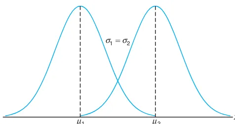
Onceµandσare specified, the normal curve is completely determined. For exam-ple, ifµ= 50 andσ= 5, then the ordinatesn(x; 50,5) can be computed for various values ofxand the curve drawn. In Figure 6.3, we have sketched two normal curves having the same standard deviation but different means. The two curves are iden-tical in form but are centered at different positions along the horizontal axis.
x 1 ⫽ 2
σ σ
1 µ2
µ
x
1 ⫽ 2 1
2
µ µ
σ σ
Figure 6.4: Normal curves withµ1=µ2andσ1< σ2.
In Figure 6.4, we have sketched two normal curves with the same mean but different standard deviations. This time we see that the two curves are centered at exactly the same position on the horizontal axis, but the curve with the larger standard deviation is lower and spreads out farther. Remember that the area under a probability curve must be equal to 1, and therefore the more variable the set of observations, the lower and wider the corresponding curve will be.
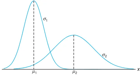
Figure 6.5 shows two normal curves having different means and different stan-dard deviations. Clearly, they are centered at different positions on the horizontal axis and their shapes reflect the two different values of σ.
x
1
2
2
µ
1
µ σ
σ
Figure 6.5: Normal curves withµ1< µ2andσ1< σ2.
Based on inspection of Figures 6.2 through 6.5 and examination of the first and second derivatives of n(x;µ, σ), we list the following properties of the normal curve:
1. The mode, which is the point on the horizontal axis where the curve is a maximum, occurs at x=µ.
2. The curve is symmetric about a vertical axis through the mean µ.
3. The curve has its points of inflection atx=µ±σ; it is concave downward if
6.2 Normal Distribution 175
4. The normal curve approaches the horizontal axis asymptotically as we proceed in either direction away from the mean.
5. The total area under the curve and above the horizontal axis is equal to 1.
Theorem 6.2: The mean and variance of n(x;µ, σ) areµand σ2, respectively. Hence, the stan-dard deviation isσ.
Proof:To evaluate the mean, we first calculate
E(X−µ) =
since the integrand above is an odd function ofz. Using Theorem 4.5 on page 128, we conclude that
E(X) =µ.
The variance of the normal distribution is given by
E[(X−µ)2] = √1
Many random variables have probability distributions that can be described adequately by the normal curve once µand σ2 are specified. In this chapter, we shall assume that these two parameters are known, perhaps from previous inves-tigations. Later, we shall make statistical inferences whenµand σ2 are unknown and have been estimated from the available experimental data.
We pointed out earlier the role that the normal distribution plays as a reason-able approximation of scientific varireason-ables in real-life experiments. There are other applications of the normal distribution that the reader will appreciate as he or she moves on in the book. The normal distribution finds enormous application as a
estimation and hypothesis testing. Theory in the important areas such as analysis of variance (Chapters 13, 14, and 15) and quality control (Chapter 17) is based on assumptions that make use of the normal distribution.
In Section 6.3, examples demonstrate the use of tables of the normal distribu-tion. Section 6.4 follows with examples of applications of the normal distribudistribu-tion.
6.3
Areas under the Normal Curve
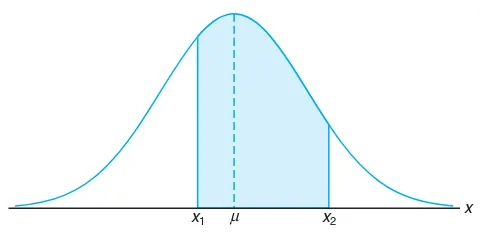
The curve of any continuous probability distribution or density function is con-structed so that the area under the curve bounded by the two ordinates x =x1 and x= x2 equals the probability that the random variableX assumes a value betweenx=x1 andx=x2. Thus, for the normal curve in Figure 6.6,
P(x1< X < x2) = x2
x1
n(x;µ, σ)dx= √1
2πσ
x2
x1
e−2σ12(x−µ)2dx
is represented by the area of the shaded region.
x
x1 µ x2
Figure 6.6: P(x1< X < x2) = area of the shaded region.
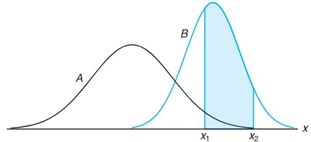
In Figures 6.3, 6.4, and 6.5 we saw how the normal curve is dependent on the mean and the standard deviation of the distribution under investigation. The area under the curve between any two ordinates must then also depend on the valuesµ andσ. This is evident in Figure 6.7, where we have shaded regions cor-responding to P(x1< X < x2) for two curves with different means and variances.
P(x1 < X < x2), where X is the random variable describing distribution A, is indicated by the shaded area below the curve ofA. IfXis the random variable de-scribing distributionB, thenP(x1< X < x2) is given by the entire shaded region. Obviously, the two shaded regions are different in size; therefore, the probability associated with each distribution will be different for the two given values ofX.
6.3 Areas under the Normal Curve 177
x
x1 x2
A
B
Figure 6.7: P(x1< X < x2) for different normal curves.
of a normal random variableZ with mean 0 and variance 1. This can be done by means of the transformation
Z= X−µ
σ .
WheneverX assumes a value x, the corresponding value of Z is given byz= (x−µ)/σ. Therefore, if X falls between the values x = x1 and x = x2, the random variableZ will fall between the corresponding valuesz1= (x1−µ)/σ and
z2= (x2−µ)/σ. Consequently, we may write
P(x1< X < x2) = 1
√
2πσ
x2
x1
e−2σ12(x−µ)2dx=√1
2π
z2
z1
e−12z2
dz
= z2
z1
n(z; 0,1)dz=P(z1< Z < z2),
whereZ is seen to be a normal random variable with mean 0 and variance 1.
Definition 6.1: The distribution of a normal random variable with mean 0 and variance 1 is called
astandard normal distribution.
The original and transformed distributions are illustrated in Figure 6.8. Since all the values ofX falling betweenx1andx2have correspondingzvalues between
z1andz2, the area under theX-curve between the ordinatesx=x1andx=x2in Figure 6.8 equals the area under the Z-curve between the transformed ordinates
z=z1andz=z2.
We have now reduced the required number of tables of normal-curve areas to one, that of the standard normal distribution. Table A.3 indicates the area under the standard normal curve corresponding toP(Z < z) for values ofzranging from
−3.49 to 3.49. To illustrate the use of this table, let us find the probability thatZis less than 1.74. First, we locate a value ofzequal to 1.7 in the left column; then we move across the row to the column under 0.04, where we read 0.9591. Therefore,
x µ
x1 x2
σ
σ
z
0 z1 z2
⫽ 1
Figure 6.8: The original and transformed normal distributions.
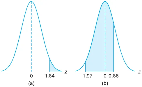
Example 6.2: Given a standard normal distribution, find the area under the curve that lies
(a) to the right ofz= 1.84 and (b) betweenz=−1.97 andz= 0.86.
z
0 1.84 (a)
z
⫺1.97 0 0.86
(b)
Figure 6.9: Areas for Example 6.2.
Solution:See Figure 6.9 for the specific areas.
(a) The area in Figure 6.9(a) to the right ofz= 1.84 is equal to 1 minus the area in Table A.3 to the left ofz= 1.84, namely, 1−0.9671 = 0.0329.
6.3 Areas under the Normal Curve 179
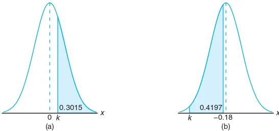
Example 6.3: Given a standard normal distribution, find the value ofksuch that
(a) P(Z > k) = 0.3015 and (b) P(k < Z <−0.18) = 0.4197.
x
0 k
(a) 0.3015
x
k −0.18
(b) 0.4197
Figure 6.10: Areas for Example 6.3.
Solution:Distributions and the desired areas are shown in Figure 6.10.
(a) In Figure 6.10(a), we see that the k value leaving an area of 0.3015 to the right must then leave an area of 0.6985 to the left. From Table A.3 it follows thatk= 0.52.
(b) From Table A.3 we note that the total area to the left of−0.18 is equal to 0.4286. In Figure 6.10(b), we see that the area betweenkand−0.18 is 0.4197, so the area to the left of k must be 0.4286−0.4197 = 0.0089. Hence, from Table A.3, we havek=−2.37.
Example 6.4: Given a random variableX having a normal distribution withµ= 50 andσ= 10, find the probability that X assumes a value between 45 and 62.
x 0
⫺0.5 1.2
Figure 6.11: Area for Example 6.4.
Solution:Thezvalues corresponding tox1= 45 andx2= 62 are
z1= 45−50
10 =−0.5 andz2=
Therefore,
P(45< X <62) =P(−0.5< Z <1.2).
P(−0.5< Z <1.2) is shown by the area of the shaded region in Figure 6.11. This area may be found by subtracting the area to the left of the ordinate z =−0.5 from the entire area to the left ofz= 1.2. Using Table A.3, we have
P(45< X <62) =P(−0.5< Z <1.2) =P(Z <1.2)−P(Z <−0.5) = 0.8849−0.3085 = 0.5764.
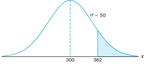
Example 6.5: Given that X has a normal distribution with µ = 300 and σ = 50, find the probability thatX assumes a value greater than 362.
Solution: The normal probability distribution with the desired area shaded is shown in Figure 6.12. To findP(X >362), we need to evaluate the area under the normal curve to the right of x= 362. This can be done by transforming x= 362 to the correspondingzvalue, obtaining the area to the left ofzfrom Table A.3, and then subtracting this area from 1. We find that
z= 362−300
50 = 1.24. Hence,
P(X >362) =P(Z >1.24) = 1−P(Z <1.24) = 1−0.8925 = 0.1075.
x
300 362
⫽ 50
σ
Figure 6.12: Area for Example 6.5.
According to Chebyshev’s theorem on page 137, the probability that a random variable assumes a value within 2 standard deviations of the mean is at least 3/4. If the random variable has a normal distribution, the z values corresponding to
x1=µ−2σand x2=µ+ 2σare easily computed to be
z1=
(µ−2σ)−µ
σ =−2 andz2=
(µ+ 2σ)−µ
σ = 2.
Hence,
P(µ−2σ < X < µ+ 2σ) =P(−2< Z <2) =P(Z <2)−P(Z <−2) = 0.9772−0.0228 = 0.9544,
6.3 Areas under the Normal Curve 181
Using the Normal Curve in Reverse
Sometimes, we are required to find the value of z corresponding to a specified probability that falls between values listed in Table A.3 (see Example 6.6). For convenience, we shall always choose thezvalue corresponding to the tabular prob-ability that comes closest to the specified probprob-ability.
The preceding two examples were solved by going first from a value ofxto az
value and then computing the desired area. In Example 6.6, we reverse the process and begin with a known area or probability, find thez value, and then determine
xby rearranging the formula
z=x−µ
σ to give x=σz+µ.
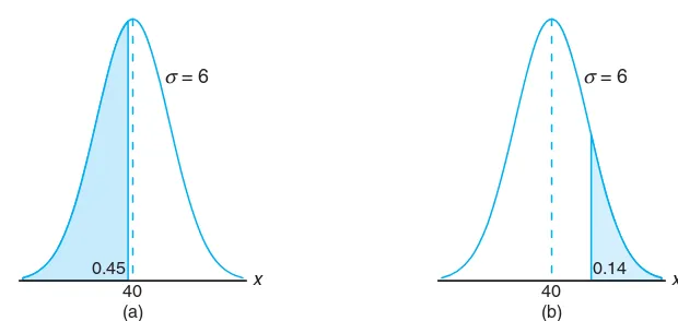
Example 6.6: Given a normal distribution withµ= 40 andσ= 6, find the value ofxthat has
(a) 45% of the area to the left and (b) 14% of the area to the right.
x 40
(a)
σ= 6 σ= 6
0.45
x 40
(b) 0.14
Figure 6.13: Areas for Example 6.6.
Solution: (a) An area of 0.45 to the left of the desiredxvalue is shaded in Figure 6.13(a).
We require a z value that leaves an area of 0.45 to the left. From Table A.3 we findP(Z <−0.13) = 0.45, so the desiredz value is−0.13. Hence,
x= (6)(−0.13) + 40 = 39.22.
(b) In Figure 6.13(b), we shade an area equal to 0.14 to the right of the desired
x value. This time we require az value that leaves 0.14 of the area to the right and hence an area of 0.86 to the left. Again, from Table A.3, we find
P(Z <1.08) = 0.86, so the desiredzvalue is 1.08 and
6.4
Applications of the Normal Distribution
Some of the many problems for which the normal distribution is applicable are treated in the following examples. The use of the normal curve to approximate binomial probabilities is considered in Section 6.5.
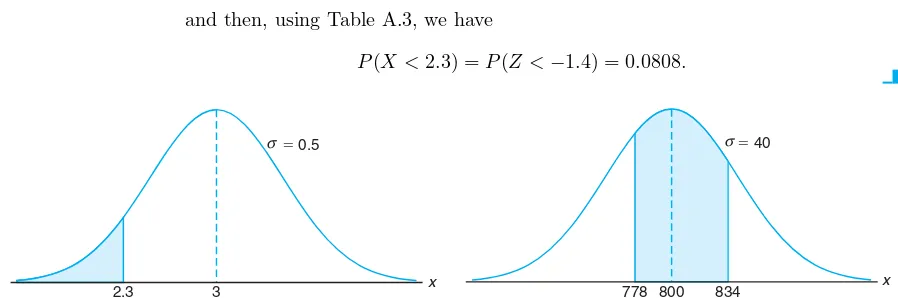
Example 6.7: A certain type of storage battery lasts, on average, 3.0 years with a standard deviation of 0.5 year. Assuming that battery life is normally distributed, find the probability that a given battery will last less than 2.3 years.
Solution: First construct a diagram such as Figure 6.14, showing the given distribution of battery lives and the desired area. To find P(X <2.3), we need to evaluate the area under the normal curve to the left of 2.3. This is accomplished by finding the area to the left of the corresponding zvalue. Hence, we find that
z= 2.3−3
0.5 =−1.4,
and then, using Table A.3, we have
P(X <2.3) =P(Z <−1.4) = 0.0808.
x 3
2.3
⫽ 0.5
σ
Figure 6.14: Area for Example 6.7.
x 800
778 834
⫽ 40
σ
Figure 6.15: Area for Example 6.8.
Example 6.8: An electrical firm manufactures light bulbs that have a life, before burn-out, that is normally distributed with mean equal to 800 hours and a standard deviation of 40 hours. Find the probability that a bulb burns between 778 and 834 hours.
Solution:The distribution of light bulb life is illustrated in Figure 6.15. Thezvalues corre-sponding tox1= 778 andx2= 834 are
z1=
778−800
40 =−0.55 andz2=
834−800
40 = 0.85.
Hence,
P(778< X <834) =P(−0.55< Z <0.85) =P(Z <0.85)−P(Z <−0.55) = 0.8023−0.2912 = 0.5111.
6.4 Applications of the Normal Distribution 183
implication is that no part falling outside these specifications will be accepted. It is known that in the process the diameter of a ball bearing has a normal distribu-tion with meanµ= 3.0 and standard deviationσ= 0.005. On average, how many manufactured ball bearings will be scrapped?
Solution:The distribution of diameters is illustrated by Figure 6.16. The values correspond-ing to the specification limits arex1 = 2.99 andx2 = 3.01. The correspondingz values are
z1=2.99−3.0
0.005 =−2.0 andz2=
3.01−3.0
0.005 = +2.0. Hence,
P(2.99< X <3.01) =P(−2.0< Z <2.0).
From Table A.3,P(Z <−2.0) = 0.0228. Due to symmetry of the normal distribu-tion, we find that
P(Z <−2.0) +P(Z >2.0) = 2(0.0228) = 0.0456.
As a result, it is anticipated that, on average, 4.56% of manufactured ball bearings will be scrapped.
x 3.0
2.99 3.01
σ= 0.005
0.0228 0.0228
Figure 6.16: Area for Example 6.9.
x 1.500
1.108 1.892
σ= 0.2
0.025 0.025
Figure 6.17: Specifications for Example 6.10.
Example 6.10: Gauges are used to reject all components for which a certain dimension is not within the specification 1.50 ± d. It is known that this measurement is normally distributed with mean 1.50 and standard deviation 0.2. Determine the value d
such that the specifications “cover” 95% of the measurements.
Solution:From Table A.3 we know that
P(−1.96< Z <1.96) = 0.95.
Therefore,
1.96 =(1.50 +d)−1.50 0.2 ,
from which we obtain
d= (0.2)(1.96) = 0.392.
Example 6.11: A certain machine makes electrical resistors having a mean resistance of 40 ohms and a standard deviation of 2 ohms. Assuming that the resistance follows a normal distribution and can be measured to any degree of accuracy, what percentage of resistors will have a resistance exceeding 43 ohms?
Solution: A percentage is found by multiplying the relative frequency by 100%. Since the relative frequency for an interval is equal to the probability of a value falling in the interval, we must find the area to the right ofx= 43 in Figure 6.18. This can be done by transforming x= 43 to the correspondingz value, obtaining the area to the left ofz from Table A.3, and then subtracting this area from 1. We find
z= 43−40 2 = 1.5. Therefore,
P(X >43) =P(Z >1.5) = 1−P(Z <1.5) = 1−0.9332 = 0.0668.
Hence, 6.68% of the resistors will have a resistance exceeding 43 ohms.
x 40 43
⫽ 2.0
σ
Figure 6.18: Area for Example 6.11.
x 40 43.5
⫽ 2.0
σ
Figure 6.19: Area for Example 6.12.
Example 6.12: Find the percentage of resistances exceeding 43 ohms for Example 6.11 if resistance is measured to the nearest ohm.
Solution:This problem differs from that in Example 6.11 in that we now assign a measure-ment of 43 ohms to all resistors whose resistances are greater than 42.5 and less than 43.5. We are actually approximating a discrete distribution by means of a continuous normal distribution. The required area is the region shaded to the right of 43.5 in Figure 6.19. We now find that
z=43.5−40
2 = 1.75. Hence,
P(X >43.5) =P(Z >1.75) = 1−P(Z <1.75) = 1−0.9599 = 0.0401.
/ /
Exercises 185
Example 6.13: The average grade for an exam is 74, and the standard deviation is 7. If 12% of the class is given As, and the grades are curved to follow a normal distribution, what is the lowest possibleA and the highest possibleB?
Solution:In this example, we begin with a known area of probability, find thez value, and then determine x from the formulax =σz+µ. An area of 0.12, corresponding to the fraction of students receivingAs, is shaded in Figure 6.20. We require az
value that leaves 0.12 of the area to the right and, hence, an area of 0.88 to the left. From Table A.3,P(Z <1.18) has the closest value to 0.88, so the desired z
value is 1.18. Hence,
x= (7)(1.18) + 74 = 82.26.
Therefore, the lowestAis 83 and the highestB is 82.
x 74
σ = 7
0.12
Figure 6.20: Area for Example 6.13.
x 74D6
σ= 7
0.6
Figure 6.21: Area for Example 6.14.
Example 6.14: Refer to Example 6.13 and find the sixth decile.
Solution:The sixth decile, writtenD6, is thexvalue that leaves 60% of the area to the left, as shown in Figure 6.21. From Table A.3 we findP(Z <0.25)≈0.6, so the desired
z value is 0.25. Nowx= (7)(0.25) + 74 = 75.75. Hence,D6= 75.75. That is, 60% of the grades are 75 or less.
Exercises
6.1 Given a continuous uniform distribution, show that
(a)µ=A+B
2 and
(b)σ2=(B−A)2
12 .
6.2 SupposeX follows a continuous uniform distribu-tion from 1 to 5. Determine the condidistribu-tional probability P(X >2.5|X≤4).
6.3 The daily amount of coffee, in liters, dispensed by a machine located in an airport lobby is a random
variable X having a continuous uniform distribution withA = 7 and B = 10. Find the probability that on a given day the amount of coffee dispensed by this machine will be
(a) at most 8.8 liters;
(b) more than 7.4 liters but less than 9.5 liters; (c) at least 8.5 liters.
186 Chapter 6 Some Continuous Probability Distributions
(a) What is the probability that the individual waits more than 7 minutes?
(b) What is the probability that the individual waits between 2 and 7 minutes?
6.5 Given a standard normal distribution, find the area under the curve that lies
(a) to the left ofz=−1.39;
6.6 Find the value of z if the area under a standard normal curve
(a) to the right ofzis 0.3622; (b) to the left ofzis 0.1131;
(c) between 0 andz, withz >0, is 0.4838; (d) between−z andz, withz >0, is 0.9500.
6.7 Given a standard normal distribution, find the value ofksuch that
(a)P(Z > k) = 0.2946; (b)P(Z < k) = 0.0427;
(c)P(−0.93< Z < k) = 0.7235.
6.8 Given a normal distribution with µ = 30 and σ= 6, find
(a) the normal curve area to the right ofx= 17; (b) the normal curve area to the left ofx= 22; (c) the normal curve area betweenx= 32 andx= 41; (d) the value of x that has 80% of the normal curve
area to the left;
(e) the two values ofxthat contain the middle 75% of the normal curve area.
6.9 Given the normally distributed variable X with mean 18 and standard deviation 2.5, find
(a)P(X <15);
(b) the value ofksuch that P(X < k) = 0.2236; (c) the value ofksuch that P(X > k) = 0.1814; (d)P(17< X <21).
6.10 According to Chebyshev’s theorem, the proba-bility that any random variable assumes a value within 3 standard deviations of the mean is at least 8/9. If it is known that the probability distribution of a random variable X is normal with mean µ and variance σ2, what is the exact value ofP(µ−3σ < X < µ+ 3σ)?
6.11 A soft-drink machine is regulated so that it dis-charges an average of 200 milliliters per cup. If the amount of drink is normally distributed with a stan-dard deviation equal to 15 milliliters,
(a) what fraction of the cups will contain more than 224 milliliters?
(b) what is the probability that a cup contains between 191 and 209 milliliters?
(c) how many cups will probably overflow if 230-milliliter cups are used for the next 1000 drinks? (d) below what value do we get the smallest 25% of the
drinks?
6.12 The loaves of rye bread distributed to local stores by a certain bakery have an average length of 30 centimeters and a standard deviation of 2 centimeters. Assuming that the lengths are normally distributed, what percentage of the loaves are
(a) longer than 31.7 centimeters?
(b) between 29.3 and 33.5 centimeters in length? (c) shorter than 25.5 centimeters?
6.13 A research scientist reports that mice will live an average of 40 months when their diets are sharply re-stricted and then enriched with vitamins and proteins. Assuming that the lifetimes of such mice are normally distributed with a standard deviation of 6.3 months, find the probability that a given mouse will live (a) more than 32 months;
(b) less than 28 months; (c) between 37 and 49 months.
6.14 The finished inside diameter of a piston ring is normally distributed with a mean of 10 centimeters and a standard deviation of 0.03 centimeter.
(a) What proportion of rings will have inside diameters exceeding 10.075 centimeters?
(b) What is the probability that a piston ring will have an inside diameter between 9.97 and 10.03 centime-ters?
(c) Below what value of inside diameter will 15% of the piston rings fall?
6.15 A lawyer commutes daily from his suburban home to his midtown office. The average time for a one-way trip is 24 minutes, with a standard deviation of 3.8 minutes. Assume the distribution of trip times to be normally distributed.
(a) What is the probability that a trip will take at least 1/2 hour?
6.5 Normal Approximation to the Binomial 187
(c) If he leaves the house at 8:35 A.M. and coffee is served at the office from 8:50A.M.until 9:00A.M., what is the probability that he misses coffee? (d) Find the length of time above which we find the
slowest 15% of the trips.
(e) Find the probability that 2 of the next 3 trips will take at least 1/2 hour.
6.16 In the November 1990 issue of Chemical Engi-neering Progress, a study discussed the percent purity of oxygen from a certain supplier. Assume that the mean was 99.61 with a standard deviation of 0.08. As-sume that the distribution of percent purity was ap-proximately normal.
(a) What percentage of the purity values would you expect to be between 99.5 and 99.7?
(b) What purity value would you expect to exceed ex-actly 5% of the population?
6.17 The average life of a certain type of small motor is 10 years with a standard deviation of 2 years. The manufacturer replaces free all motors that fail while under guarantee. If she is willing to replace only 3% of the motors that fail, how long a guarantee should be offered? Assume that the lifetime of a motor follows a normal distribution.
6.18 The heights of 1000 students are normally dis-tributed with a mean of 174.5 centimeters and a stan-dard deviation of 6.9 centimeters. Assuming that the heights are recorded to the nearest half-centimeter, how many of these students would you expect to have heights
(a) less than 160.0 centimeters?
(b) between 171.5 and 182.0 centimeters inclusive? (c) equal to 175.0 centimeters?
(d) greater than or equal to 188.0 centimeters?
6.19 A company pays its employees an average wage of $15.90 an hour with a standard deviation of $1.50. If the wages are approximately normally distributed and paid to the nearest cent,
(a) what percentage of the workers receive wages be-tween $13.75 and $16.22 an hour inclusive? (b) the highest 5% of the employee hourly wages is
greater than what amount?
6.20 The weights of a large number of miniature poo-dles are approximately normally distributed with a mean of 8 kilograms and a standard deviation of 0.9 kilogram. If measurements are recorded to the nearest tenth of a kilogram, find the fraction of these poodles with weights
(a) over 9.5 kilograms; (b) of at most 8.6 kilograms;
(c) between 7.3 and 9.1 kilograms inclusive.
6.21 The tensile strength of a certain metal compo-nent is normally distributed with a mean of 10,000 kilo-grams per square centimeter and a standard deviation of 100 kilograms per square centimeter. Measurements are recorded to the nearest 50 kilograms per square centimeter.
(a) What proportion of these components exceed 10,150 kilograms per square centimeter in tensile strength?
(b) If specifications require that all components have tensile strength between 9800 and 10,200 kilograms per square centimeter inclusive, what proportion of pieces would we expect to scrap?
6.22 If a set of observations is normally distributed, what percent of these differ from the mean by (a) more than 1.3σ?
(b) less than 0.52σ?
6.23 The IQs of 600 applicants to a certain college are approximately normally distributed with a mean of 115 and a standard deviation of 12. If the college requires an IQ of at least 95, how many of these stu-dents will be rejected on this basis of IQ, regardless of their other qualifications? Note that IQs are recorded to the nearest integers.
6.5
Normal Approximation to the Binomial
are discrete. The first application of a continuous probability distribution to ap-proximate probabilities over a discrete sample space was demonstrated in Example 6.12, where the normal curve was used. The normal distribution is often a good approximation to a discrete distribution when the latter takes on a symmetric bell shape. From a theoretical point of view, some distributions converge to the normal as their parameters approach certain limits. The normal distribution is a conve-nient approximating distribution because the cumulative distribution function is so easily tabled. The binomial distribution is nicely approximated by the normal in practical problems when one works with the cumulative distribution function. We now state a theorem that allows us to use areas under the normal curve to approximate binomial properties when nis sufficiently large.
Theorem 6.3: If X is a binomial random variable with mean µ =np and variance σ2 = npq, then the limiting form of the distribution of
Z= X√−np
npq ,
asn→ ∞, is the standard normal distributionn(z; 0,1).
It turns out that the normal distribution withµ=npand σ2=np(1−p) not only provides a very accurate approximation to the binomial distribution when
n is large and pis not extremely close to 0 or 1 but also provides a fairly good approximation even whennis small andpis reasonably close to 1/2.
To illustrate the normal approximation to the binomial distribution, we first draw the histogram for b(x; 15,0.4) and then superimpose the particular normal curve having the same mean and variance as the binomial variable X. Hence, we draw a normal curve with
µ=np= (15)(0.4) = 6 andσ2=npq= (15)(0.4)(0.6) = 3.6.
The histogram of b(x; 15,0.4) and the corresponding superimposed normal curve, which is completely determined by its mean and variance, are illustrated in Figure 6.22.
11
0 1 2 3 4 5 6 7 8 9 13 15 x
6.5 Normal Approximation to the Binomial 189
The exact probability that the binomial random variable X assumes a given valuexis equal to the area of the bar whose base is centered atx. For example, the exact probability that X assumes the value 4 is equal to the area of the rectangle with base centered atx= 4. Using Table A.1, we find this area to be
P(X= 4) =b(4; 15,0.4) = 0.1268,
which is approximately equal to the area of the shaded region under the normal curve between the two ordinatesx1= 3.5 andx2= 4.5 in Figure 6.23. Converting to zvalues, we have
z1= 3.5−6
1.897 =−1.32 and z2= 4.5−6
1.897 =−0.79.
11
0 1 2 3 4 5 6 7 8 9 13 15 x
Figure 6.23: Normal approximation ofb(x; 15,0.4) and 9
x=7
b(x; 15,0.4).
IfX is a binomial random variable andZ a standard normal variable, then
P(X= 4) =b(4; 15,0.4)≈P(−1.32< Z <−0.79)
=P(Z <−0.79)−P(Z <−1.32) = 0.2148−0.0934 = 0.1214.
This agrees very closely with the exact value of 0.1268.
The normal approximation is most useful in calculating binomial sums for large values of n. Referring to Figure 6.23, we might be interested in the probability that X assumes a value from 7 to 9 inclusive. The exact probability is given by
P(7≤X ≤9) = 9
x=0
b(x; 15,0.4)−
6
x=0
b(x; 15,0.4)
= 0.9662−0.6098 = 0.3564,
which is equal to the sum of the areas of the rectangles with bases centered at
x = 7, 8, and 9. For the normal approximation, we find the area of the shaded region under the curve between the ordinatesx1= 6.5 andx2= 9.5 in Figure 6.23. The correspondingz values are
z1= 6.5−6
1.897 = 0.26 and z2= 9.5−6
Now,
P(7≤X ≤9)≈P(0.26< Z <1.85) =P(Z <1.85)−P(Z <0.26) = 0.9678−0.6026 = 0.3652.
Once again, the normal curve approximation provides a value that agrees very closely with the exact value of 0.3564. The degree of accuracy, which depends on how well the curve fits the histogram, will increase asnincreases. This is particu-larly true whenpis not very close to 1/2 and the histogram is no longer symmetric. Figures 6.24 and 6.25 show the histograms forb(x; 6,0.2) andb(x; 15,0.2), respec-tively. It is evident that a normal curve would fit the histogram considerably better whenn= 15 than whenn= 6.
0 1 2 3 4 5 6 x
Figure 6.24: Histogram forb(x; 6,0.2).
0 1 2 3 4 5 6 7 8 9 11 13 15 x
Figure 6.25: Histogram forb(x; 15,0.2).
In our illustrations of the normal approximation to the binomial, it became apparent that if we seek the area under the normal curve to the left of, say, x, it is more accurate to use x+ 0.5. This is a correction to accommodate the fact that a discrete distribution is being approximated by a continuous distribution. The correction+0.5is called acontinuity correction. The foregoing discussion leads to the following formal normal approximation to the binomial.
Normal Approximation to the Binomial Distribution
LetX be a binomial random variable with parametersnandp. For largen,X
has approximately a normal distribution withµ=npandσ2=npq=np(1−p) and
P(X ≤x) =
x
k=0
b(k;n, p)
≈ area under normal curve to the left ofx+ 0.5
= P
Z ≤x+ 0√.npq5−np
,
and the approximation will be good ifnpandn(1−p) are greater than or equal to 5.
As we indicated earlier, the quality of the approximation is quite good for large
6.5 Normal Approximation to the Binomial 191
approximation. Both the normal approximation and the true binomial cumulative probabilities are given. Notice that atp= 0.05 andp= 0.10, the approximation is fairly crude for n = 10. However, even for n= 10, note the improvement for
p= 0.50. On the other hand, whenpis fixed at p= 0.05, note the improvement of the approximation as we go fromn= 20 ton= 100.
Table 6.1: Normal Approximation and True Cumulative Binomial Probabilities
p= 0.05, n= 10 p= 0.10, n= 10 p= 0.50, n= 10
r Binomial Normal Binomial Normal Binomial Normal
0 0.5987 0.5000 0.3487 0.2981 0.0010 0.0022 1 0.9139 0.9265 0.7361 0.7019 0.0107 0.0136 2 0.9885 0.9981 0.9298 0.9429 0.0547 0.0571 3 0.9990 1.0000 0.9872 0.9959 0.1719 0.1711 4 1.0000 1.0000 0.9984 0.9999 0.3770 0.3745
5 1.0000 1.0000 0.6230 0.6255
6 0.8281 0.8289
7 0.9453 0.9429
8 0.9893 0.9864
9 0.9990 0.9978
10 1.0000 0.9997
p= 0.05
n= 20 n= 50 n= 100
r Binomial Normal Binomial Normal Binomial Normal
0 0.3585 0.3015 0.0769 0.0968 0.0059 0.0197 1 0.7358 0.6985 0.2794 0.2578 0.0371 0.0537 2 0.9245 0.9382 0.5405 0.5000 0.1183 0.1251 3 0.9841 0.9948 0.7604 0.7422 0.2578 0.2451 4 0.9974 0.9998 0.8964 0.9032 0.4360 0.4090 5 0.9997 1.0000 0.9622 0.9744 0.6160 0.5910 6 1.0000 1.0000 0.9882 0.9953 0.7660 0.7549
7 0.9968 0.9994 0.8720 0.8749
8 0.9992 0.9999 0.9369 0.9463
9 0.9998 1.0000 0.9718 0.9803
10 1.0000 1.0000 0.9885 0.9941
Example 6.15: The probability that a patient recovers from a rare blood disease is 0.4. If 100 people are known to have contracted this disease, what is the probability that fewer than 30 survive?
Solution:Let the binomial variableX represent the number of patients who survive. Since
n= 100, we should obtain fairly accurate results using the normal-curve approxi-mation with
µ=np= (100)(0.4) = 40 andσ=√npq=(100)(0.4)(0.6) = 4.899.
Thez value corresponding to 29.5 is
z= 29.5−40
4.899 =−2.14,
and the probability of fewer than 30 of the 100 patients surviving is given by the shaded region in Figure 6.26. Hence,
P(X <30)≈P(Z <−2.14) = 0.0162.
0
⫺2.14
x
⫽ 1
σ
Figure 6.26: Area for Example 6.15.
0 1.16 2.71 x
⫽ 1
σ
Figure 6.27: Area for Example 6.16.
Example 6.16: A multiple-choice quiz has 200 questions, each with 4 possible answers of which only 1 is correct. What is the probability that sheer guesswork yields from 25 to 30 correct answers for the 80 of the 200 problems about which the student has no knowledge?
Solution:The probability of guessing a correct answer for each of the 80 questions isp= 1/4. IfX represents the number of correct answers resulting from guesswork, then
P(25≤X ≤30) = 30
x=25
b(x; 80,1/4).
Using the normal curve approximation with
µ=np= (80) 1
4
= 20
and
σ=√npq=(80)(1/4)(3/4) = 3.873,
we need the area between x1 = 24.5 and x2 = 30.5. The corresponding z values are
z1=
24.5−20
3.873 = 1.16 andz2=
30.5−20
3.873 = 2.71.
The probability of correctly guessing from 25 to 30 questions is given by the shaded region in Figure 6.27. From Table A.3 we find that
P(25≤X ≤30) = 30
x=25
b(x; 80,0.25)≈P(1.16< Z <2.71)
/ /
Exercises 193
Exercises
6.24 A coin is tossed 400 times. Use the normal curve approximation to find the probability of obtaining (a) between 185 and 210 heads inclusive;
(b) exactly 205 heads;
(c) fewer than 176 or more than 227 heads.
6.25 A process for manufacturing an electronic com-ponent yields items of which 1% are defective. A qual-ity control plan is to select 100 items from the process, and if none are defective, the process continues. Use the normal approximation to the binomial to find (a) the probability that the process continues given the
sampling plan described;
(b) the probability that the process continues even if the process has gone bad (i.e., if the frequency of defective components has shifted to 5.0% defec-tive).
6.26 A process yields 10% defective items. If 100 items are randomly selected from the process, what is the probability that the number of defectives (a) exceeds 13?
(b) is less than 8?
6.27 The probability that a patient recovers from a delicate heart operation is 0.9. Of the next 100 patients having this operation, what is the probability that (a) between 84 and 95 inclusive survive?
(b) fewer than 86 survive?
6.28 Researchers at George Washington University and the National Institutes of Health claim that ap-proximately 75% of people believe “tranquilizers work very well to make a person more calm and relaxed.” Of the next 80 people interviewed, what is the probability that
(a) at least 50 are of this opinion? (b) at most 56 are of this opinion?
6.29 If 20% of the residents in a U.S. city prefer a white telephone over any other color available, what is the probability that among the next 1000 telephones installed in that city
(a) between 170 and 185 inclusive will be white? (b) at least 210 but not more than 225 will be white?
6.30 A drug manufacturer claims that a certain drug cures a blood disease, on the average, 80% of the time. To check the claim, government testers use the drug on
a sample of 100 individuals and decide to accept the claim if 75 or more are cured.
(a) What is the probability that the claim will be re-jected when the cure probability is, in fact, 0.8? (b) What is the probability that the claim will be
ac-cepted by the government when the cure probabil-ity is as low as 0.7?
6.31 One-sixth of the male freshmen entering a large state school are out-of-state students. If the students are assigned at random to dormitories, 180 to a build-ing, what is the probability that in a given dormitory at least one-fifth of the students are from out of state?
6.32 A pharmaceutical company knows that approx-imately 5% of its birth-control pills have an ingredient that is below the minimum strength, thus rendering the pill ineffective. What is the probability that fewer than 10 in a sample of 200 pills will be ineffective?
6.33 Statistics released by the National Highway Traffic Safety Administration and the National Safety Council show that on an average weekend night, 1 out of every 10 drivers on the road is drunk. If 400 drivers are randomly checked next Saturday night, what is the probability that the number of drunk drivers will be (a) less than 32?
(b) more than 49?
(c) at least 35 but less than 47?
6.34 A pair of dice is rolled 180 times. What is the probability that a total of 7 occurs
(a) at least 25 times?
(b) between 33 and 41 times inclusive? (c) exactly 30 times?
6.35 A company produces component parts for an en-gine. Parts specifications suggest that 95% of items meet specifications. The parts are shipped to cus-tomers in lots of 100.
(a) What is the probability that more than 2 items in a given lot will be defective?
(b) What is the probability that more than 10 items in a lot will be defective?
tick-ets were sold. What is the probability that the airline overbooked this flight?
6.37 The serum cholesterol level X in 14-year-old boys has approximately a normal distribution with mean 170 and standard deviation 30.
(a) Find the probability that the serum cholesterol level of a randomly chosen 14-year-old boy exceeds 230.
(b) In a middle school there are 300 14-year-old boys. Find the probability that at least 8 boys have a serum cholesterol level that exceeds 230.
6.38 A telemarketing company has a special letter-opening machine that opens and removes the contents of an envelope. If the envelope is fed improperly into the machine, the contents of the envelope may not be removed or may be damaged. In this case, the machine is said to have “failed.”
(a) If the machine has a probability of failure of 0.01, what is the probability of more than 1 failure oc-curring in a batch of 20 envelopes?
(b) If the probability of failure of the machine is 0.01 and a batch of 500 envelopes is to be opened, what is the probability that more than 8 failures will occur?
6.6
Gamma and Exponential Distributions
Although the normal distribution can be used to solve many problems in engineer-ing and science, there are still numerous situations that require different types of density functions. Two such density functions, the gamma and exponential distributions, are discussed in this section.
It turns out that the exponential distribution is a special case of the gamma dis-tribution. Both find a large number of applications. The exponential and gamma distributions play an important role in both queuing theory and reliability prob-lems. Time between arrivals at service facilities and time to failure of component parts and electrical systems often are nicely modeled by the exponential distribu-tion. The relationship between the gamma and the exponential allows the gamma to be used in similar types of problems. More details and illustrations will be supplied later in the section.
The gamma distribution derives its name from the well-knowngamma func-tion, studied in many areas of mathematics. Before we proceed to the gamma distribution, let us review this function and some of its important properties.
Definition 6.2: Thegamma functionis defined by
Γ(α) = ∞
0
xα−1e−xdx, forα >0.
The following are a few simple properties of the gamma function. (a) Γ(n) = (n−1)(n−2)· · ·(1)Γ(1), for a positive integern.
forα >1, which yields the recursion formula
Γ(α) = (α−1)Γ(α−1).
6.6 Gamma and Exponential Distributions 195
(b) Γ(n) = (n−1)! for a positive integern. (c) Γ(1) = 1.
Furthermore, we have the following property of Γ(α), which is left for the reader to verify (see Exercise 6.39 on page 206).
(d) Γ(1/2) =√π.
The following is the definition of thegamma distribution.
Gamma Distribution
The continuous random variableX has agamma distribution, with param-etersαandβ, if its density function is given by
f(x;α, β) = 1
βαΓ(α)xα−1e−x/β, x >0,
0, elsewhere,
whereα >0 andβ >0.
Graphs of several gamma distributions are shown in Figure 6.28 for certain specified values of the parameters α and β. The special gamma distribution for whichα= 1 is called theexponential distribution.
0 1 2 3 4 5 6
0.5 1.0
f(x)
x = 1
α β= 1
= 2
α β= 1
= 4
α β= 1
Figure 6.28: Gamma distributions.
Exponential Distribution
The continuous random variable X has an exponential distribution, with parameterβ, if its density function is given by
f(x;β) = 1
βe−x/β, x >0,
0, elsewhere,
The following theorem and corollary give the mean and variance of the gamma and exponential distributions.
Theorem 6.4: The mean and variance of the gamma distribution are
µ=αβ andσ2=αβ2.
The proof of this theorem is found in Appendix A.26.
Corollary 6.1: The mean and variance of the exponential distribution are
µ=β andσ2=β2.
Relationship to the Poisson Process
We shall pursue applications of the exponential distribution and then return to the gamma distribution. The most important applications of the exponential distribu-tion are situadistribu-tions where the Poisson process applies (see Secdistribu-tion 5.5). The reader should recall that the Poisson process allows for the use of the discrete distribu-tion called the Poisson distribudistribu-tion. Recall that the Poisson distribudistribu-tion is used to compute the probability of specific numbers of “events” during a particularperiod of time or span of space. In many applications, the time period or span of space is the random variable. For example, an industrial engineer may be interested in modeling the timeT between arrivals at a congested intersection during rush hour in a large city. An arrival represents the Poisson event.
The relationship between the exponential distribution (often called the negative exponential) and the Poisson process is quite simple. In Chapter 5, the Poisson distribution was developed as a single-parameter distribution with parameter λ, where λmay be interpreted as the mean number of eventsper unit “time.” Con-sider now the random variable described by the time required for the first event to occur. Using the Poisson distribution, we find that the probability of no events occurring in the span up to time tis given by
p(0;λt) = e
−λt(λt)0
0! =e −λt.
We can now make use of the above and let X be the time to the first Poisson event. The probability that the length of time until the first event will exceedxis the same as the probability that no Poisson events will occur inx. The latter, of course, is given bye−λx. As a result,
P(X > x) =e−λx.
Thus, the cumulative distribution function forX is given by
P(0≤X ≤x) = 1−e−λx.
6.6 Gamma and Exponential Distributions 197
function
f(x) =λe−λx,
which is the density function of the exponential distribution withλ= 1/β.
Applications of the Exponential and Gamma Distributions
In the foregoing, we provided the foundation for the application of the exponential distribution in “time to arrival” or time to Poisson event problems. We will illus-trate some applications here and then proceed to discuss the role of the gamma distribution in these modeling applications. Notice that the mean of the exponen-tial distribution is the parameterβ, the reciprocal of the parameter in the Poisson distribution. The reader should recall that it is often said that the Poisson distri-bution has no memory, implying that occurrences in successive time periods are independent. The important parameter β is the mean time between events. In reliability theory, where equipment failure often conforms to this Poisson process,
β is calledmean time between failures. Many equipment breakdowns do follow the Poisson process, and thus the exponential distribution does apply. Other ap-plications include survival times in biomedical experiments and computer response time.
In the following example, we show a simple application of the exponential dis-tribution to a problem in reliability. The binomial disdis-tribution also plays a role in the solution.
Example 6.17: Suppose that a system contains a certain type of component whose time, in years, to failure is given byT. The random variableTis modeled nicely by the exponential distribution with mean time to failureβ = 5. If 5 of these components are installed in different systems, what is the probability that at least 2 are still functioning at the end of 8 years?
Solution: The probability that a given component is still functioning after 8 years is given by
P(T >8) = 1 5
∞
8
e−t/5 dt=e−8/5
≈0.2.
LetX represent the number of components functioning after 8 years. Then using the binomial distribution, we have
P(X ≥2) = 5
x=2
b(x; 5,0.2) = 1−
1
x=0
b(x; 5,0.2) = 1−0.7373 = 0.2627.
There are exercises and examples in Chapter 3 where the reader has already encountered the exponential distribution. Others involving waiting time and reli-ability include Example 6.24 and some of the exercises and review exercises at the end of this chapter.
The Memoryless Property and Its Effect on the Exponential Distribution
say, an electronic component where lifetime has an exponential distribution, the probability that the component lasts, say,t hours, that is, P(X ≥t), is the same as the conditional probability
P(X ≥t0+t|X ≥t0).
So if the component “makes it” tot0hours, the probability of lasting an additional
t hours is the same as the probability of lasting t hours. There is no “punish-ment” through wear that may have ensued for lasting the first t0 hours. Thus, the exponential distribution is more appropriate when the memoryless property is justified. But if the failure of the component is a result of gradual or slow wear (as in mechanical wear), then the exponential does not apply and either the gamma or the Weibull distribution (Section 6.10) may be more appropriate.
The importance of the gamma distribution lies in the fact that it defines a family of which other distributions are special cases. But the gamma itself has important applications in waiting time and reliability theory. Whereas the expo-nential distribution describes the time until the occurrence of a Poisson event (or the time between Poisson events), the time (or space) occurring until a specified number of Poisson events occur is a random variable whose density function is described by the gamma distribution. This specific number of events is the param-eter αin the gamma density function. Thus, it becomes easy to understand that when α= 1, the special case of the exponential distribution occurs. The gamma density can be developed from its relationship to the Poisson process in much the same manner as we developed the exponential density. The details are left to the reader. The following is a numerical example of the use of the gamma distribution in a waiting-time application.
Example 6.18: Suppose that telephone calls arriving at a particular switchboard follow a Poisson process with an average of 5 calls coming per minute. What is the probability that up to a minute will elapse by the time 2 calls have come in to the switchboard?
Solution: The Poisson process applies, with time until 2 Poisson events following a gamma distribution with β = 1/5 and α = 2. Denote by X the time in minutes that transpires before 2 calls come. The required probability is given by
P(X ≤1) = 1
0 1
β2xe−
x/β dx= 25
1
0
xe−5xdx= 1−e−5(1 + 5) = 0.96.
While the origin of the gamma distribution deals in time (or space) until the occurrence of αPoisson events, there are many instances where a gamma distri-bution works very well even though there is no clear Poisson structure. This is particularly true for survival timeproblems in both engineering and biomedical applications.
6.6 Gamma and Exponential Distributions 199
Solution: Let the random variable X be the survival time (time to death). The required probability is
The integral above can be solved through the use of the incomplete gamma function, which becomes the cumulative distribution function for the gamma dis-tribution. This function is written as
F(x;α) =
which is denoted as F(6; 5) in the table of the incomplete gamma function in Appendix A.23. Note that this allows a quick computation of probabilities for the gamma distribution. Indeed, for this problem, the probability that the rat survives no longer than 60 days is given by
P(X≤60) =F(6; 5) = 0.715.
Example 6.20: It is known, from previous data, that the length of time in months between cus-tomer complaints about a certain product is a gamma distribution with α = 2 andβ= 4. Changes were made to tighten quality control requirements. Following these changes, 20 months passed before the first complaint. Does it appear as if the quality control tightening was effective?
Solution: Let X be the time to the first complaint, which, under conditions prior to the changes, followed a gamma distribution with α = 2 and β = 4. The question centers around how rareX ≥20 is, given that αand β remain at values 2 and 4, respectively. In other words, under the prior conditions is a “time to complaint” as large as 20 months reasonable? Thus, following the solution to Example 6.19,
P(X≥20) = 1−β1α
As a result, we could conclude that the conditions of the gamma distribution with α = 2 and β = 4 are not supported by the data that an observed time to complaint is as large as 20 months. Thus, it is reasonable to conclude that the quality control work was effective.
Example 6.21: Consider Exercise 3.31 on page 94. Based on extensive testing, it is determined that the time Y in years before a major repair is required for a certain washing machine is characterized by the density function
f(y) = 1
4e−
Note thatY is an exponential random variable withµ= 4 years. The machine is considered a bargain if it is unlikely to require a major repair before the sixth year. What is the probabilityP(Y >6)? What is the probability that a major repair is required in the first year?
Solution:Consider the cumulative distribution functionF(y) for the exponential distribution,
F(y) = 1
β
y
0
e−t/β dt= 1
−e−y/β.
Then
P(Y >6) = 1−F(6) =e−3/2= 0.2231.
Thus, the probability that the washing machine will require major repair after year six is 0.223. Of course, it will require repair before year six with probability 0.777. Thus, one might conclude the machine is not really a bargain. The probability that a major repair is necessary in the first year is
P(Y <1) = 1−e−1/4= 1
−0.779 = 0.221.
6.7
Chi-Squared Distribution
Another very important special case of the gamma distribution is obtained by letting α=v/2 andβ = 2, wherev is a positive integer. The result is calledthe chi-squared distribution. The distribution has a single parameter,v, called the
degrees of freedom.
Chi-Squared Distribution
The continuous random variable X has a chi-squared distribution, withv
degrees of freedom, if its density function is given by
f(x;v) = 1
2v/2Γ(v/2)x
v/2−1e−x/2, x >0,
0, elsewhere,
wherev is a positive integer.
The chi-squared distribution plays a vital role in statistical inference. It has considerable applications in both methodology and theory. While we do not discuss applications in detail in this chapter, it is important to understand that Chapters 8, 9, and 16 contain important applications. The chi-squared distribution is an important component of statistical hypothesis testing and estimation.
Topics dealing with sampling distributions, analysis of variance, and nonpara-metric statistics involve extensive use of the chi-squared distribution.
Theorem 6.5: The mean and variance of the chi-squared distribution are
6.9 Lognormal Distribution 201
6.8
Beta Distribution
An extension to the uniform distribution is a beta distribution. Let us start by defining abeta function.
Definition 6.3: Abeta functionis defined by
B(α, β) = 1
0
xα−1(1
−x)β−1dx= Γ(α)Γ(β)
Γ(α+β), forα, β >0,
where Γ(α) is the gamma function.
Beta Distribution The continuous random variableX has abeta distribution with parameters
α >0 andβ >0 if its density function is given by
f(x) = 1
B(α,β)xα−1(1−x)β−1, 0< x <1,
0, elsewhere.
Note that the uniform distribution on (0,1) is a beta distribution with parameters
α= 1 andβ = 1.
Theorem 6.6: The mean and variance of a beta distribution with parameters αandβ are
µ= α
α+β andσ
2= αβ
(α+β)2(α+β+ 1),
respectively.
For the uniform distribution on (0,1), the mean and variance are
µ= 1
1 + 1 = 1 2 andσ
2= (1)(1)
(1 + 1)2(1 + 1 + 1)= 1 12,
respectively.
6.9
Lognormal Distribution
The lognormal distribution is used for a wide variety of applications. The dis-tribution applies in cases where a natural log transformation results in a normal distribution.
Lognormal Distribution
The continuous random variableX has alognormal distribution if the ran-dom variableY = ln(X) has a normal distribution with mean µand standard deviationσ. The resulting density function ofX is
f(x;µ, σ) = 1
√ 2πσxe
−2σ12[ln(x)−µ]2, x≥0,
0.2 0.4 0.6 f(x)
x
µ σ
= 0 = 1
µ σ
= 1 = 1
0 1 2 3 4 5
Figure 6.29: Lognormal distributions.
The graphs of the lognormal distributions are illustrated in Figure 6.29.
Theorem 6.7: The mean and variance of the lognormal distribution are
µ=eµ+σ2/2 andσ2=e2µ+σ2(eσ2−1).
The cumulative distribution function is quite simple due to its relationship to the normal distribution. The use of the distribution function is illustrated by the following example.
Example 6.22: Concentrations of pollutants produced by chemical plants historically are known to exhibit behavior that resembles a lognormal distribution. This is important when one considers issues regarding compliance with government regulations. Suppose it is assumed that the concentration of a certain pollutant, in parts per million, has a lognormal distribution with parameters µ = 3.2 and σ = 1. What is the probability that the concentration exceeds 8 parts per million?
Solution:Let the random variable X be pollutant concentration. Then
P(X >8) = 1−P(X ≤8).
Since ln(X) has a normal distribution with meanµ= 3.2 and standard deviation
σ= 1,
P(X ≤8) = Φ ln(8)
−3.2 1
= Φ(−1.12) = 0.1314.
6.10 Weibull Distribution (Optional) 203
Example 6.23: The life, in thousands of miles, of a certain type of electronic control for locomotives has an approximately lognormal distribution withµ= 5.149 andσ= 0.737. Find the 5th percentile of the life of such an electronic control.
Solution: From Table A.3, we know that P(Z < −1.645) = 0.05. Denote by X the life of such an electronic control. Since ln(X) has a normal distribution with mean
µ= 5.149 andσ= 0.737, the 5th percentile ofX can be calculated as
ln(x) = 5.149 + (0.737)(−1.645) = 3.937.
Hence,x= 51.265. This means that only 5% of the controls will have lifetimes less than 51,265 miles.
6.10
Weibull Distribution (Optional)
Modern technology has enabled engineers to design many complicated systems whose operation and safety depend on the reliability of the various components making up the systems. For example, a fuse may burn out, a steel column may buckle, or a heat-sensing device may fail. Identical components subjected to iden-tical environmental conditions will fail at different and unpredictable times. We have seen the role that the gamma and exponential distributions play in these types of problems. Another distribution that has been used extensively in recent years to deal with such problems is theWeibull distribution, introduced by the Swedish physicist Waloddi Weibull in 1939.
Weibull Distribution
The continuous random variableX has aWeibull distribution, with param-etersαandβ, if its density function is given by
f(x;α, β) =
The graphs of the Weibull distribution forα= 1 and various values of the param-eter β are illustrated in Figure 6.30. We see that the curves change considerably in shape for different values of the parameter β. If we letβ = 1, the Weibull dis-tribution reduces to the exponential disdis-tribution. For values ofβ >1, the curves become somewhat bell shaped and resemble the normal curve but display some skewness.
The mean and variance of the Weibull distribution are stated in the following theorem. The reader is asked to provide the proof in Exercise 6.52 on page 206.
Theorem 6.8: The mean and variance of the Weibull distribution are
µ=α−1/βΓ
0 0.5 1.0 1.5 2.0
f(x)
x
⫽ 1 ⫽ 2
⫽ 3.5
β
β β
Figure 6.30: Weibull distributions (α= 1).
life length of a component, measured from some specified time until it fails. Let us represent this time to failure by the continuous random variable T, with probability density function f(t), where f(t) is the Weibull distribution. The Weibull distribution has inherent flexibility in that it does not require the lack of memory property of the exponential distribution. The cumulative distribution function (cdf) for the Weibull can be written in closed form and certainly is useful in computing probabilities.
cdf for Weibull Distribution
The cumulative distribution function for the Weibull distribution is given by
F(x) = 1−e−αxβ
, forx≥0,
forα >0 andβ >0.
Example 6.24: The length of lifeX, in hours, of an item in a machine shop has a Weibull distri-bution with α= 0.01 andβ = 2. What is the probability that it fails before eight hours of usage?
Solution:P(X <8) =F(8) = 1−e−(0.01)82
= 1−0.527 = 0.473.
The Failure Rate for the Weibull Distribution
6.10 Weibull Distribution (Optional) 205
the reliability of the given component at timet, we may write
R(t) =P(T > t) = ∞
t
f(t)dt= 1−F(t),
whereF(t) is the cumulative distribution function ofT. The conditional probability that a component will fail in the interval from T =t toT =t+ ∆t, given that it survived to timet, is
F(t+ ∆t)−F(t)
R(t) .
Dividing this ratio by ∆tand taking the limit as ∆t→0, we get thefailure rate, denoted byZ(t). Hence,
Z(t) = lim ∆t→0
F(t+ ∆t)−F(t) ∆t
1
R(t) =
F′(t) R(t) =
f(t)
R(t) =
f(t) 1−F(t),
which expresses the failure rate in terms of the distribution of the time to failure. SinceZ(t) =f(t)/[1−F(t)], the failure rate is given as follows:
Failure Rate for Weibull Distribution
Thefailure rate at timet for the Weibull distribution is given by
Z(t) =αβtβ−1, t >0.
Interpretation of the Failure Rate
The quantityZ(t) is aptly named as a failure rate since it does quantify the rate of change over time of the conditional probability that the component lasts an additional ∆t given that it has lasted to time t. The rate of decrease (or increase) with time is important. The following are crucial points.
(a) Ifβ = 1, the failure rate =α, a constant. This, as indicated earlier, is the special case of the exponential distribution in which lack of memory prevails. (b) If β > 1, Z(t) is an increasing function of time t, which indicates that the
component wears over time.
(c) If β < 1, Z(t) is a decreasing function of time t and hence the component strengthens or hardens over time.
For example, the item in the machine shop in Example 6.24 has β = 2, and hence it wears over time. In fact, the failure rate function is given byZ(t) = 0.02t. On the other hand, suppose the parameters wereβ= 3/4 andα= 2. In that case,
206 Chapter 6 Some Continuous Probability Distributions
Exercises
6.39 Use the gamma function withy=√2xto show that Γ(1/2) =√π.
6.40 In a certain city, the daily consumption of water (in millions of liters) follows approximately a gamma distribution withα= 2 andβ= 3. If the daily capac-ity of that ccapac-ity is 9 million liters of water, what is the probability that on any given day the water supply is inadequate?
6.41 If a random variableX has the gamma distribu-tion withα= 2 andβ= 1, findP(1.8< X <2.4).
6.42 Suppose that the time, in hours, required to repair a heat pump is a random variable X having a gamma distribution with parameters α = 2 and β = 1/2. What is the probability that on the next service call
(a) at most 1 hour will be required to repair the heat pump?
(b) at least 2 hours will be required to repair the heat pump?
6.43 (a) Find the mean and variance of the daily wa-ter consumption in Exercise 6.40.
(b) According to Chebyshev’s theorem, there is a prob-ability of at least 3/4 that the water consumption on any given day will fall within what interval?
6.44 In a certain city, the daily consumption of elec-tric power, in millions of kilowatt-hours, is a random variable X having a gamma distribution with mean µ= 6 and varianceσ2= 12.
(a) Find the values ofαandβ.
(b) Find the probability that on any given day the daily power consumption will exceed 12 million kilowatt-hours.
6.45 The length of time for one individual to be served at a cafeteria is a random variable having an ex-ponential distribution with a mean of 4 minutes. What is the probability that a person is served in less than 3 minutes on at least 4 of the next 6 days?
6.46 The life, in years, of a certain type of electrical switch has an exponential distribution with an average lifeβ= 2. If 100 of these switches are installed in dif-ferent systems, what is the probability that at most 30 fail during the first year?
6.47 Suppose that the service life, in years, of a hear-ing aid battery is a random variable havhear-ing a Weibull distribution withα= 1/2 andβ= 2.
(a) How long can such a battery be expected to last? (b) What is the probability that such a battery will be
operating after 2 years?
6.48 Derive the mean and variance of the beta distri-bution.
6.49 Suppose the random variable X follows a beta distribution withα= 1 andβ= 3.
(a) Determine the mean and median ofX. (b) Determine the variance ofX.
(c) Find the probability thatX >1/3.
6.50 If the proportion of a brand of television set re-quiring service during the first year of operation is a random variable having a beta distribution withα= 3 andβ= 2, what is the probability that at least 80% of the new models of this brand sold this year will require service during their first year of operation?
6.51 The lives of a certain automobile seal have the Weibull distribution with failure rate Z(t) =1/√t. Find the probability that such a seal is still intact after 4 years.
6.52 Derive the mean and variance of the Weibull dis-tribution.
6.53 In a biomedical research study, it was deter-mined that the survival time, in weeks, of an animal subjected to a certain exposure of gamma radiation has a gamma distribution withα= 5 andβ= 10. (a) What is the mean survival time of a randomly
se-lected animal of the type used in the experiment? (b) What is the standard deviation of survival time?
(c) What is the probability that an animal survives more than 30 weeks?
6.54 The lifetime, in weeks, of a certain type of tran-sistor is known to follow a gamma distribution with mean 10 weeks and standard deviation√50 weeks. (a) What is the probability that a transistor of this
type will last at most 50 weeks?
(b) What is the probability that a transistor of this type will not survive the first 10 weeks?
![Figure 6.1: The density function for a random variable on the interval [1, 3].](https://thumb-ap.123doks.com/thumbv2/123dok/2188134.1617974/3.520.187.427.69.207/figure-density-function-random-variable-interval.webp)