Probability & Statistics for
Engineers & Scientists
N I N T H
E D I T I O N
Ronald E. Walpole
Roanoke College
Raymond H. Myers
Virginia Tech
Sharon L. Myers
Radford University
Keying Ye
University of Texas at San Antonio
Chapter 9
One- and Two-Sample
Estimation Problems
9.1
Introduction
In previous chapters, we emphasized sampling properties of the sample mean and variance. We also emphasized displays of data in various forms. The purpose of these presentations is to build a foundation that allows us to draw conclusions about the population parameters from experimental data. For example, the Central Limit Theorem provides information about the distribution of the sample mean ¯X. The distribution involves the population meanµ. Thus, any conclusions concerning µ
drawn from an observed sample average must depend on knowledge of this sampling distribution. Similar comments apply toS2 and σ2. Clearly, any conclusions we
draw about the variance of a normal distribution will likely involve the sampling distribution ofS2.
In this chapter, we begin by formally outlining the purpose of statistical in-ference. We follow this by discussing the problem of estimation of population parameters. We confine our formal developments of specific estimation proce-dures to problems involving one and two samples.
9.2
Statistical Inference
In Chapter 1, we discussed the general philosophy of formal statistical inference.
Statistical inferenceconsists of those methods by which one makes inferences or generalizations about a population. The trend today is to distinguish between the
classical method of estimating a population parameter, whereby inferences are based strictly on information obtained from a random sample selected from the population, and theBayesian method, which utilizes prior subjective knowledge about the probability distribution of the unknown parameters in conjunction with the information provided by the sample data. Throughout most of this chapter, we shall use classical methods to estimate unknown population parameters such as the mean, the proportion, and the variance by computing statistics from random
samples and applying the theory of sampling distributions, much of which was covered in Chapter 8. Bayesian estimation will be discussed in Chapter 18.
Statistical inference may be divided into two major areas: estimation and
tests of hypotheses. We treat these two areas separately, dealing with theory and applications of estimation in this chapter and hypothesis testing in Chapter 10. To distinguish clearly between the two areas, consider the following examples. A candidate for public office may wish to estimate the true proportion of voters favoring him by obtaining opinions from a random sample of 100 eligible voters. The fraction of voters in the sample favoring the candidate could be used as an estimate of the true proportion in the population of voters. A knowledge of the sampling distribution of a proportion enables one to establish the degree of accuracy of such an estimate. This problem falls in the area of estimation.
Now consider the case in which one is interested in finding out whether brand
A floor wax is more scuff-resistant than brand B floor wax. He or she might hypothesize that brandAis better than brandBand, after proper testing, accept or reject this hypothesis. In this example, we do not attempt to estimate a parameter, but instead we try to arrive at a correct decision about a prestated hypothesis. Once again we are dependent on sampling theory and the use of data to provide us with some measure of accuracy for our decision.
9.3
Classical Methods of Estimation
Apoint estimateof some population parameterθis a single value ˆθof a statistic ˆ
Θ. For example, the value ¯xof the statistic ¯X, computed from a sample of sizen, is a point estimate of the population parameter µ. Similarly, ˆp=x/n is a point estimate of the true proportionpfor a binomial experiment.
An estimator is not expected to estimate the population parameter without error. We do not expect ¯X to estimateµexactly, but we certainly hope that it is not far off. For a particular sample, it is possible to obtain a closer estimate of µ
by using the sample median ˜X as an estimator. Consider, for instance, a sample consisting of the values 2, 5, and 11 from a population whose mean is 4 but is supposedly unknown. We would estimate µto be ¯x= 6, using the sample mean as our estimate, or ˜x= 5, using the sample median as our estimate. In this case, the estimator ˜X produces an estimate closer to the true parameter than does the estimator ¯X. On the other hand, if our random sample contains the values 2, 6, and 7, then ¯x= 5 and ˜x= 6, so ¯X is the better estimator. Not knowing the true value ofµ, we must decide in advance whether to use ¯X or ˜X as our estimator.
Unbiased Estimator
9.3 Classical Methods of Estimation 267
Definition 9.1: A statistic ˆΘ is said to be anunbiased estimator of the parameterθif
µΘˆ =E( ˆΘ) =θ.
Example 9.1: Show thatS2 is an unbiased estimator of the parameterσ2. Solution:In Section 8.5 on page 244, we showed that
n
i=1
(Xi−X¯)2= n
i=1
(Xi−µ)2−n( ¯X−µ)2.
Now
E(S2) =E
1
n−1
n
i=1
(Xi−X¯)2
= 1
n−1
n
i=1
E(Xi−µ)2−nE( ¯X−µ)2
= 1
n−1
n
i=1
σ2 Xi−nσ
2 ¯ X
.
However,
σ2Xi=σ
2, fori= 1,2, . . . , n, andσ2 ¯ X =
σ2
n.
Therefore,
E(S2) = 1
n−1
nσ2−nσ2
n
=σ2.
AlthoughS2is an unbiased estimator ofσ2,S, on the other hand, is usually a
biased estimator ofσ, with the bias becoming insignificant for large samples. This example illustrateswhy we divide byn
−1rather thannwhen the variance is
estimated.
Variance of a Point Estimator
If ˆΘ1and ˆΘ2 are two unbiased estimators of the same population parameterθ, we
want to choose the estimator whose sampling distribution has the smaller variance. Hence, if σθ2ˆ1< σ2θˆ2, we say that ˆΘ1 is amore efficient estimatorofθthan ˆΘ2.
Definition 9.2: If we consider all possible unbiased estimators of some parameterθ, the one with
the smallest variance is called themost efficient estimatorofθ.
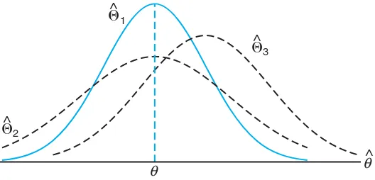
Figure 9.1 illustrates the sampling distributions of three different estimators, ˆ
Θ1, ˆΘ2, and ˆΘ3, all estimating θ. It is clear that only ˆΘ1 and ˆΘ2 are unbiased,
since their distributions are centered atθ. The estimator ˆΘ1has a smaller variance
than ˆΘ2 and is therefore more efficient. Hence, our choice for an estimator ofθ,
among the three considered, would be ˆΘ1.
θ
^
θ
^2
^1
^3
Figure 9.1: Sampling distributions of different estimators ofθ.
of ˜X. Thus, both estimates ¯xand ˜xwill, on average, equal the population mean
µ, but ¯xis likely to be closer toµfor a given sample, and thus ¯X is more efficient than ˜X.
Interval Estimation
Even the most efficient unbiased estimator is unlikely to estimate the population parameter exactly. It is true that estimation accuracy increases with large samples, but there is still no reason we should expect apoint estimatefrom a given sample to be exactly equal to the population parameter it is supposed to estimate. There are many situations in which it is preferable to determine an interval within which we would expect to find the value of the parameter. Such an interval is called an
interval estimate.
An interval estimate of a population parameter θ is an interval of the form ˆ
θL < θ < θˆU, where ˆθL and ˆθU depend on the value of the statistic ˆΘ for a
particular sample and also on the sampling distribution of ˆΘ. For example, a random sample of SAT verbal scores for students in the entering freshman class might produce an interval from 530 to 550, within which we expect to find the true average of all SAT verbal scores for the freshman class. The values of the endpoints, 530 and 550, will depend on the computed sample mean ¯x and the sampling distribution of ¯X. As the sample size increases, we know thatσ2
¯ X=σ
2/n
decreases, and consequently our estimate is likely to be closer to the parameterµ, resulting in a shorter interval. Thus, the interval estimate indicates, by its length, the accuracy of the point estimate. An engineer will gain some insight into the population proportion defective by taking a sample and computing the sample proportion defective. But an interval estimate might be more informative.
Interpretation of Interval Estimates
Since different samples will generally yield different values of ˆΘ and, therefore, different values for ˆθL and ˆθU, these endpoints of the interval are values of
corre-sponding random variables ˆΘL and ˆΘU. From the sampling distribution of ˆΘ we
9.4 Single Sample: Estimating the Mean 269
positive fractional value we care to specify. If, for instance, we find ˆΘL and ˆΘU
such that
P( ˆΘL< θ <ΘˆU) = 1−α,
for 0< α <1, then we have a probability of 1−αof selecting a random sample that will produce an interval containing θ. The interval ˆθL < θ <θˆU, computed from
the selected sample, is called a 100(1−α)% confidence interval, the fraction 1−α is called the confidence coefficient or the degree of confidence, and the endpoints, ˆθL and ˆθU, are called the lower and upper confidence limits.
Thus, when α= 0.05, we have a 95% confidence interval, and whenα= 0.01, we obtain a wider 99% confidence interval. The wider the confidence interval is, the more confident we can be that the interval contains the unknown parameter. Of course, it is better to be 95% confident that the average life of a certain television transistor is between 6 and 7 years than to be 99% confident that it is between 3 and 10 years. Ideally, we prefer a short interval with a high degree of confidence. Sometimes, restrictions on the size of our sample prevent us from achieving short intervals without sacrificing some degree of confidence.
In the sections that follow, we pursue the notions of point and interval esti-mation, with each section presenting a different special case. The reader should notice that while point and interval estimation represent different approaches to gaining information regarding a parameter, they are related in the sense that con-fidence interval estimators are based on point estimators. In the following section, for example, we will see that ¯X is a very reasonable point estimator of µ. As a result, the important confidence interval estimator of µdepends on knowledge of the sampling distribution of ¯X.
We begin the following section with the simplest case of a confidence interval. The scenario is simple and yet unrealistic. We are interested in estimating a popu-lation meanµand yetσis known. Clearly, ifµis unknown, it is quite unlikely that
σis known. Any historical results that produced enough information to allow the assumption thatσis known would likely have produced similar information about
µ. Despite this argument, we begin with this case because the concepts and indeed the resulting mechanics associated with confidence interval estimation remain the same for the more realistic situations presented later in Section 9.4 and beyond.
9.4
Single Sample: Estimating the Mean
The sampling distribution of ¯X is centered at µ, and in most applications the variance is smaller than that of any other estimators of µ. Thus, the sample mean ¯xwill be used as a point estimate for the population mean µ. Recall that
σ2 ¯ X =σ
2/n, so a large sample will yield a value of ¯X that comes from a sampling
distribution with a small variance. Hence, ¯xis likely to be a very accurate estimate ofµwhennis large.
Let us now consider the interval estimate of µ. If our sample is selected from a normal population or, failing this, if n is sufficiently large, we can establish a confidence interval forµby considering the sampling distribution of ¯X.
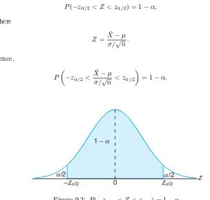
standard deviationσX¯ =σ/√n. Writingzα/2 for thez-value above which we find
an area of α/2 under the normal curve, we can see from Figure 9.2 that
P(−zα/2< Z < zα/2) = 1−α,
where
Z= X¯ −µ
σ/√n.
Hence,
P
−zα/2<
¯
X−µ σ/√n < zα/2
= 1−α.
z 1−
−zα/2 0 zα/2
α/2 α/2
α
Figure 9.2: P(−zα/2< Z < zα/2) = 1−α.
Multiplying each term in the inequality byσ/√nand then subtracting ¯Xfrom each term and multiplying by −1 (reversing the sense of the inequalities), we obtain
P
¯
X−zα/2
σ
√
n < µ <X¯+zα/2 σ
√
n
= 1−α.
A random sample of sizenis selected from a population whose varianceσ2is known,
and the mean ¯xis computed to give the 100(1−α)% confidence interval below. It is important to emphasize that we have invoked the Central Limit Theorem above. As a result, it is important to note the conditions for applications that follow.
Confidence Interval onµ,σ2
Known
If ¯xis the mean of a random sample of size nfrom a population with known varianceσ2, a 100(1−α)% confidence interval forµis given by
¯
x−zα/2
σ
√
n < µ <¯x+zα/2 σ
√
n,
wherezα/2 is thez-value leaving an area of α/2 to the right.
9.4 Single Sample: Estimating the Mean 271
the shape of the distributions not too skewed, sampling theory guarantees good results.
Clearly, the values of the random variables ˆΘLand ˆΘU, defined in Section 9.3,
are the confidence limits
ˆ
θL= ¯x−zα/2
σ
√
n and θˆU = ¯x+zα/2 σ
√
n.
Different samples will yield different values of ¯x and therefore produce different interval estimates of the parameter µ, as shown in Figure 9.3. The dot at the center of each interval indicates the position of the point estimate ¯xfor that random sample. Note that all of these intervals are of the same width, since their widths depend only on the choice of zα/2 once ¯xis determined. The larger the value we
choose for zα/2, the wider we make all the intervals and the more confident we
can be that the particular sample selected will produce an interval that contains the unknown parameterµ. In general, for a selection ofzα/2, 100(1−α)% of the
intervals will coverµ.
1 2 3 4 5 6 7 8 9 10
µ x
Sample
Figure 9.3: Interval estimates ofµfor different samples.
Example 9.2: The average zinc concentration recovered from a sample of measurements taken in 36 different locations in a river is found to be 2.6 grams per milliliter. Find the 95% and 99% confidence intervals for the mean zinc concentration in the river. Assume that the population standard deviation is 0.3 gram per milliliter.
Solution: The point estimate of µ is ¯x= 2.6. Thez-value leaving an area of 0.025 to the
right, and therefore an area of 0.975 to the left, isz0.025= 1.96 (Table A.3). Hence,
the 95% confidence interval is
2.6−(1.96)
0.3 √
36
< µ <2.6 + (1.96)
0.3 √
36
which reduces to 2.50< µ <2.70. To find a 99% confidence interval, we find the
z-value leaving an area of 0.005 to the right and 0.995 to the left. From Table A.3 again,z0.005= 2.575, and the 99% confidence interval is
2.6−(2.575)
0.3
√ 36
< µ <2.6 + (2.575)
0.3
√ 36
,
or simply
2.47< µ <2.73.
We now see that a longer interval is required to estimateµwith a higher degree of confidence.
The 100(1−α)% confidence interval provides an estimate of the accuracy of our point estimate. If µis actually the center value of the interval, then ¯xestimates
µ without error. Most of the time, however, ¯xwill not be exactly equal to µand the point estimate will be in error. The size of this error will be the absolute value of the difference between µand ¯x, and we can be 100(1−α)% confident that this difference will not exceedzα/2√σn. We can readily see this if we draw a diagram of
a hypothetical confidence interval, as in Figure 9.4.
x µ
Error
x zα/2σ/ n x zα/2σ/ n
Figure 9.4: Error in estimatingµby ¯x.
Theorem 9.1: If ¯xis used as an estimate ofµ, we can be 100(1−α)% confident that the error will not exceedzα/2√σn.
In Example 9.2, we are 95% confident that the sample mean ¯x= 2.6 differs from the true mean µ by an amount less than (1.96)(0.3)/√36 = 0.1 and 99% confident that the difference is less than (2.575)(0.3)/√36 = 0.13.
Frequently, we wish to know how large a sample is necessary to ensure that the error in estimating µwill be less than a specified amounte. By Theorem 9.1, we must choose nsuch thatzα/2√σn =e. Solving this equation gives the following
formula forn.
Theorem 9.2: If ¯xis used as an estimate ofµ, we can be 100(1−α)% confident that the error will not exceed a specified amountewhen the sample size is
n=#zα/2σ
e
$2
.
9.4 Single Sample: Estimating the Mean 273
Strictly speaking, the formula in Theorem 9.2 is applicable only if we know the variance of the population from which we select our sample. Lacking this information, we could take a preliminary sample of size n ≥ 30 to provide an estimate ofσ. Then, usingsas an approximation forσ in Theorem 9.2, we could determine approximately how many observations are needed to provide the desired degree of accuracy.
Example 9.3: How large a sample is required if we want to be 95% confident that our estimate ofµin Example 9.2 is off by less than 0.05?
Solution:The population standard deviation isσ= 0.3. Then, by Theorem 9.2,
n=
(1.96)(0.3)
0.05
2
= 138.3.
Therefore, we can be 95% confident that a random sample of size 139 will provide an estimate ¯xdiffering fromµby an amount less than 0.05.
One-Sided Confidence Bounds
The confidence intervals and resulting confidence bounds discussed thus far are
two-sided(i.e., both upper and lower bounds are given). However, there are many applications in which only one bound is sought. For example, if the measurement of interest is tensile strength, the engineer receives better information from a lower bound only. This bound communicates the worst-case scenario. On the other hand, if the measurement is something for which a relatively large value ofµis not profitable or desirable, then an upper confidence bound is of interest. An example would be a case in which inferences need to be made concerning the mean mercury composition in a river. An upper bound is very informative in this case.
One-sided confidence bounds are developed in the same fashion as two-sided intervals. However, the source is a one-sided probability statement that makes use of the Central Limit Theorem:
P
X¯
−µ σ/√n < zα
= 1−α.
One can then manipulate the probability statement much as before and obtain
P(µ >X¯−zασ/√n) = 1−α.
Similar manipulation ofP#X¯−µ σ/√n >−zα
$
= 1−αgives
P(µ <X¯+zασ/√n) = 1−α.
As a result, the upper and lower one-sided bounds follow.
One-Sided Confidence Bounds onµ,σ2 Known
If ¯X is the mean of a random sample of sizenfrom a population with variance
σ2, the one-sided 100(1−α)% confidence bounds forµare given by
upper one-sided bound: x¯+zασ/√n;
Example 9.4: In a psychological testing experiment, 25 subjects are selected randomly and their reaction time, in seconds, to a particular stimulus is measured. Past experience suggests that the variance in reaction times to these types of stimuli is 4 sec2 and
that the distribution of reaction times is approximately normal. The average time for the subjects is 6.2 seconds. Give an upper 95% bound for the mean reaction time.
Solution:The upper 95% bound is given by
¯
x+zασ/√n= 6.2 + (1.645)
4/25 = 6.2 + 0.658 = 6.858 seconds.
Hence, we are 95% confident that the mean reaction time is less than 6.858 seconds.
The Case of
σ
Unknown
Frequently, we must attempt to estimate the mean of a population when the vari-ance is unknown. The reader should recall learning in Chapter 8 that if we have a random sample from anormal distribution, then the random variable
T = X¯ −µ
S/√n
has a Student t-distribution withn−1 degrees of freedom. HereS is the sample standard deviation. In this situation, withσunknown,T can be used to construct a confidence interval onµ. The procedure is the same as that withσknown except that σ is replaced by S and the standard normal distribution is replaced by the
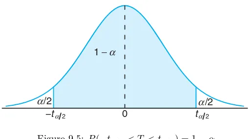
t-distribution. Referring to Figure 9.5, we can assert that
P(−tα/2< T < tα/2) = 1−α,
wheretα/2is thet-value withn−1 degrees of freedom, above which we find an area
of α/2. Because of symmetry, an equal area of α/2 will fall to the left of−tα/2.
Substituting forT, we write
P
−tα/2<
¯
X−µ S/√n < tα/2
= 1−α.
Multiplying each term in the inequality by S/√n, and then subtracting ¯X from each term and multiplying by−1, we obtain
P
¯
X−tα/2
S
√
n < µ <X¯ +tα/2 S
√
n
= 1−α.
9.4 Single Sample: Estimating the Mean 275
t
1−
−tα2 0 tα2
α/2 α/2
α
Figure 9.5: P(−tα/2< T < tα/2) = 1−α.
Confidence Interval onµ,σ2 Unknown
If ¯x and s are the mean and standard deviation of a random sample from a normal population with unknown varianceσ2, a 100(1−α)% confidence interval
forµis
¯
x−tα/2
s
√
n < µ <x¯+tα/2 s
√
n,
wheretα/2is the t-value withv =n−1 degrees of freedom, leaving an area of
α/2 to the right.
We have made a distinction between the cases of σknown andσ unknown in computing confidence interval estimates. We should emphasize that for σknown we exploited the Central Limit Theorem, whereas for σ unknown we made use of the sampling distribution of the random variable T. However, the use of thet -distribution is based on the premise that the sampling is from a normal -distribution. As long as the distribution is approximately bell shaped, confidence intervals can be computed whenσ2 is unknown by using thet-distribution and we may expect
very good results.
Computed one-sided confidence bounds forµwithσunknown are as the reader would expect, namely
¯
x+tα√s
n and x¯−tα s
√
n.
They are the upper and lower 100(1−α)% bounds, respectively. Here tα is the
t-value having an area ofαto the right.
Example 9.5: The contents of seven similar containers of sulfuric acid are 9.8, 10.2, 10.4, 9.8, 10.0, 10.2, and 9.6 liters. Find a 95% confidence interval for the mean contents of all such containers, assuming an approximately normal distribution.
Solution:The sample mean and standard deviation for the given data are
¯
x= 10.0 and s= 0.283.
95% confidence interval for µis
10.0−(2.447)
0.283 √
7
< µ <10.0 + (2.447)
0.283 √
7
,
which reduces to 9.74< µ <10.26.
Concept of a Large-Sample Confidence Interval
Often statisticians recommend that even when normality cannot be assumed,σis unknown, and n≥30,scan replaceσand the confidence interval
¯
x±zα/2
s
√n
may be used. This is often referred to as a large-sample confidence interval. The justification lies only in the presumption that with a sample as large as 30 and the population distribution not too skewed, swill be very close to the trueσand thus the Central Limit Theorem prevails. It should be emphasized that this is only an approximation and the quality of the result becomes better as the sample size grows larger.
Example 9.6: Scholastic Aptitude Test (SAT) mathematics scores of a random sample of 500 high school seniors in the state of Texas are collected, and the sample mean and standard deviation are found to be 501 and 112, respectively. Find a 99% confidence interval on the mean SAT mathematics score for seniors in the state of Texas.
Solution: Since the sample size is large, it is reasonable to use the normal approximation. Using Table A.3, we findz0.005= 2.575. Hence, a 99% confidence interval forµis
501±(2.575)
112
√ 500
= 501±12.9,
which yields 488.1< µ <513.9.
9.5
Standard Error of a Point Estimate
We have made a rather sharp distinction between the goal of a point estimate and that of a confidence interval estimate. The former supplies a single number extracted from a set of experimental data, and the latter provides an interval that is reasonable for the parameter,given the experimental data; that is, 100(1−α)% of such computed intervals “cover” the parameter.
These two approaches to estimation are related to each other. The common thread is the sampling distribution of the point estimator. Consider, for example, the estimator ¯X of µ withσ known. We indicated earlier that a measure of the quality of an unbiased estimator is its variance. The variance of ¯X is
σ2 ¯ X=
σ2
9.6 Prediction Intervals 277
Thus, the standard deviation of ¯X, orstandard errorof ¯X, is σ/√n. Simply put, the standard error of an estimator is its standard deviation. For ¯X, the computed confidence limit
¯
x±zα/2
σ
√
n is written as ¯x±zα/2 s.e.(¯x),
where “s.e.” is the “standard error.” The important point is that the width of the confidence interval onµis dependent on the quality of the point estimator through its standard error. In the case whereσis unknown and sampling is from a normal distribution,sreplacesσand theestimated standard errors/√nis involved. Thus, the confidence limits on µare
Confidence Limits onµ,σ2 Unknown
¯
x±tα/2
s
√
n = ¯x±tα/2s.e.(¯x)
Again, the confidence interval is no better(in terms of width) than the quality of the point estimate, in this case through its estimated standard error. Computer packages often refer to estimated standard errors simply as “standard errors.”
As we move to more complex confidence intervals, there is a prevailing notion that widths of confidence intervals become shorter as the quality of the correspond-ing point estimate becomes better, although it is not always quite as simple as we have illustrated here. It can be argued that a confidence interval is merely an augmentation of the point estimate to take into account the precision of the point estimate.
9.6
Prediction Intervals
The point and interval estimations of the mean in Sections 9.4 and 9.5 provide good information about the unknown parameter µ of a normal distribution or a nonnormal distribution from which a large sample is drawn. Sometimes, other than the population mean, the experimenter may also be interested in predicting the possiblevalue of a future observation. For instance, in quality control, the experimenter may need to use the observed data to predict a new observation. A process that produces a metal part may be evaluated on the basis of whether the part meets specifications on tensile strength. On certain occasions, a customer may be interested in purchasing asingle part. In this case, a confidence interval on the mean tensile strength does not capture the required information. The customer requires a statement regarding the uncertainty of asingle observation. This type of requirement is nicely fulfilled by the construction of aprediction interval.
It is quite simple to obtain a prediction interval for the situations we have considered so far. Assume that the random sample comes from a normal population with unknown mean µ and known variance σ2. A natural point estimator of a
new observation is ¯X. It is known, from Section 8.4, that the variance of ¯X is
σ2/n. However, to predict a new observation, not only do we need to account for the variation due to estimating the mean, but also we should account for the
prediction interval is best illustrated by beginning with a normal random variable
x0−x¯, where x0 is the new observation and ¯xcomes from the sample. Since x0
and ¯xare independent, we know that
z=x0−x¯
σ2+σ2/n =
x0−x¯
σ1 + 1/n
is n(z; 0,1). As a result, if we use the probability statement
P(−zα/2< Z < zα/2) = 1−α
with thez-statistic above and placex0 in the center of the probability statement,
we have the following event occurring with probability 1−α:
¯
x−zα/2σ
1 + 1/n < x0<x¯+zα/2σ
1 + 1/n.
As a result, computation of the prediction interval is formalized as follows.
Prediction Interval of a Future Observation,σ2 Known
For a normal distribution of measurements with unknown meanµ and known varianceσ2, a 100(1−α)%prediction intervalof a future observation x
0 is
¯
x−zα/2σ
1 + 1/n < x0<x¯+zα/2σ
1 + 1/n,
wherezα/2 is thez-value leaving an area of α/2 to the right.
Example 9.7: Due to the decrease in interest rates, the First Citizens Bank received a lot of mortgage applications. A recent sample of 50 mortgage loans resulted in an average loan amount of $257,300. Assume a population standard deviation of $25,000. For the next customer who fills out a mortgage application, find a 95% prediction interval for the loan amount.
Solution: The point prediction of the next customer’s loan amount is ¯x= $257,300. The
z-value here isz0.025 = 1.96. Hence, a 95% prediction interval for the future loan
amount is
257,300−(1.96)(25,000)1 + 1/50< x0<257,300 + (1.96)(25,000)
1 + 1/50,
which gives the interval ($207,812.43, $306,787.57).
9.6 Prediction Intervals 279
Prediction Interval of a Future Observation,σ2 Unknown
For a normal distribution of measurements with unknown meanµand unknown varianceσ2, a 100(1−α)% prediction intervalof a future observationx
0 is
¯
x−tα/2s
1 + 1/n < x0<x¯+tα/2s
1 + 1/n,
wheretα/2is the t-value withv =n−1 degrees of freedom, leaving an area of
α/2 to the right.
One-sided prediction intervals can also be constructed. Upper prediction bounds apply in cases where focus must be placed on future large observations. Concern over future small observations calls for the use of lower prediction bounds. The upper bound is given by
¯
x+tαs
1 + 1/n
and the lower bound by
¯
x−tαs
1 + 1/n.
Example 9.8: A meat inspector has randomly selected 30 packs of 95% lean beef. The sample resulted in a mean of 96.2% with a sample standard deviation of 0.8%. Find a 99% prediction interval for the leanness of a new pack. Assume normality.
Solution:Forv= 29 degrees of freedom,t0.005= 2.756. Hence, a 99% prediction interval for
a new observationx0 is
96.2−(2.756)(0.8)
"
1 + 1
30 < x0<96.2 + (2.756)(0.8)
"
1 + 1 30,
which reduces to (93.96, 98.44).
Use of Prediction Limits for Outlier Detection
To this point in the text very little attention has been paid to the concept of
outliers, or aberrant observations. The majority of scientific investigators are keenly sensitive to the existence of outlying observations or so-called faulty or “bad data.” We deal with the concept of outlier detection extensively in Chapter 12. However, it is certainly of interest here since there is an important relationship between outlier detection and prediction intervals.
9.7
Tolerance Limits
As discussed in Section 9.6, the scientist or engineer may be less interested in esti-mating parameters than in gaining a notion about where an individualobservation
or measurement might fall. Such situations call for the use of prediction intervals. However, there is yet a third type of interval that is of interest in many applica-tions. Once again, suppose that interest centers around the manufacturing of a component part and specifications exist on a dimension of that part. In addition, there is little concern about the mean of the dimension. But unlike in the scenario in Section 9.6, one may be less interested in a single observation and more inter-ested in where the majority of the population falls. If process specifications are important, the manager of the process is concerned about long-range performance,
not the next observation. One must attempt to determine bounds that, in some probabilistic sense, “cover” values in the population (i.e., the measured values of the dimension).
One method of establishing the desired bounds is to determine a confidence interval on a fixed proportion of the measurements. This is best motivated by visualizing a situation in which we are doing random sampling from a normal distribution with known meanµand varianceσ2. Clearly, a bound that covers the
middle 95% of the population of observations is
µ±1.96σ.
This is called a tolerance interval, and indeed its coverage of 95% of measured observations is exact. However, in practice, µ andσare seldom known; thus, the user must apply
¯
x±ks.
Now, of course, the interval is a random variable, and hence the coverage of a proportion of the population by the interval is not exact. As a result, a 100(1−γ)% confidence interval must be used since ¯x±ks cannot be expected to cover any specified proportion all the time. As a result, we have the following definition.
Tolerance Limits For a normal distribution of measurements with unknown meanµand unknown standard deviation σ, tolerance limits are given by ¯x±ks, where k is de-termined such that one can assert with 100(1−γ)% confidence that the given limits contain at least the proportion 1−αof the measurements.
Table A.7 gives values of k for 1−α = 0.90,0.95,0.99; γ = 0.05,0.01; and selected values of nfrom 2 to 300.
Example 9.9: Consider Example 9.8. With the information given, find a tolerance interval that gives two-sided 95% bounds on 90% of the distribution of packages of 95% lean beef. Assume the data came from an approximately normal distribution.
Solution:Recall from Example 9.8 thatn= 30, the sample mean is 96.2%, and the sample standard deviation is 0.8%. From Table A.7, k= 2.14. Using
¯
9.7 Tolerance Limits 281
we find that the lower and upper bounds are 94.5 and 97.9.
We are 95% confident that the above range covers the central 90% of the dis-tribution of 95% lean beef packages.
Distinction among Confidence Intervals, Prediction Intervals,
and Tolerance Intervals
It is important to reemphasize the difference among the three types of intervals dis-cussed and illustrated in the preceding sections. The computations are straightfor-ward, but interpretation can be confusing. In real-life applications, these intervals are not interchangeable because their interpretations are quite distinct.
In the case of confidence intervals, one is attentive only to the population mean. For example, Exercise 9.13 on page 283 deals with an engineering process that produces shearing pins. A specification will be set on Rockwell hardness, below which a customer will not accept any pins. Here, a population parameter must take a backseat. It is important that the engineer know where the majority of the values of Rockwell hardness are going to be. Thus, tolerance limits should be used. Surely, when tolerance limits on any process output are tighter than process specifications, that is good news for the process manager.
It is true that the tolerance limit interpretation is somewhat related to the confidence interval. The 100(1−α)% tolerance interval on, say, the proportion 0.95 can be viewed as a confidence intervalon the middle 95%of the corresponding normal distribution. One-sided tolerance limits are also relevant. In the case of the Rockwell hardness problem, it is desirable to have a lower bound of the form ¯
x−ks such that there is 99% confidence that at least 99% of Rockwell hardness values will exceed the computed value.
Prediction intervals are applicable when it is important to determine a bound on a single value. The mean is not the issue here, nor is the location of the majority of the population. Rather, the location of a single new observation is required.
Case Study 9.1: Machine Quality: A machine produces metal pieces that are cylindrical in shape. A sample of these pieces is taken and the diameters are found to be 1.01, 0.97, 1.03, 1.04, 0.99, 0.98, 0.99, 1.01, and 1.03 centimeters. Use these data to calculate three interval types and draw interpretations that illustrate the distinction between them in the context of the system. For all computations, assume an approximately normal distribution. The sample mean and standard deviation for the given data are ¯x= 1.0056 ands= 0.0246.
(a) Find a 99% confidence interval on the mean diameter.
(b) Compute a 99% prediction interval on a measured diameter of a single metal piece taken from the machine.
(c) Find the 99% tolerance limits that will contain 95% of the metal pieces pro-duced by this machine.
Solution: (a) The 99% confidence interval for the mean diameter is given by
¯
282 Chapter 9 One- and Two-Sample Estimation Problems
Thus, the 99% confidence bounds are 0.9781 and 1.0331. (b) The 99% prediction interval for a future observation is given by
¯
x±t0.005s
1 + 1/n= 1.0056±(3.355)(0.0246)1 + 1/9,
with the bounds being 0.9186 and 1.0926.
(c) From Table A.7, forn= 9, 1−γ= 0.99, and 1−α= 0.95, we findk= 4.550 for two-sided limits. Hence, the 99% tolerance limits are given by
¯
x+ks= 1.0056±(4.550)(0.0246),
with the bounds being 0.8937 and 1.1175. We are 99% confident that the tolerance interval from 0.8937 to 1.1175 will contain the central 95% of the distribution of diameters produced.
This case study illustrates that the three types of limits can give appreciably dif-ferent results even though they are all 99% bounds. In the case of the confidence interval on the mean, 99% of such intervals cover the population mean diameter. Thus, we say that we are 99% confident that the mean diameter produced by the process is between 0.9781 and 1.0331 centimeters. Emphasis is placed on the mean, with less concern about a single reading or the general nature of the distribution of diameters in the population. In the case of the prediction limits, the bounds 0.9186 and 1.0926 are based on the distribution of a single “new” metal piece taken from the process, and again 99% of such limits will cover the diameter of a new measured piece. On the other hand, the tolerance limits, as suggested in the previous section, give the engineer a sense of where the “majority,” say the central 95%, of the diameters of measured pieces in the population reside. The 99% tolerance limits, 0.8937 and 1.1175, are numerically quite different from the other two bounds. If these bounds appear alarmingly wide to the engineer, it re-flects negatively on process quality. On the other hand, if the bounds represent a desirable result, the engineer may conclude that a majority (95% in here) of the diameters are in a desirable range. Again, a confidence interval interpretation may be used: namely, 99% of such calculated bounds will cover the middle 95% of the population of diameters.
Exercises
9.1 A UCLA researcher claims that the life span of
mice can be extended by as much as 25% when the calories in their diet are reduced by approximately 40% from the time they are weaned. The restricted diet is enriched to normal levels by vitamins and protein. Assuming that it is known from previous studies that
σ = 5.8 months, how many mice should be included
in our sample if we wish to be 99% confident that the mean life span of the sample will be within 2 months of the population mean for all mice subjected to this reduced diet?
9.2 An electrical firm manufactures light bulbs that
have a length of life that is approximately normally distributed with a standard deviation of 40 hours. If a sample of 30 bulbs has an average life of 780 hours, find a 96% confidence interval for the population mean of all bulbs produced by this firm.
9.3 Many cardiac patients wear an implanted
/ /
Exercises 283
interval for the mean of the depths of all connector modules made by a certain manufacturing company. A random sample of 75 modules has an average depth of 0.310 inch.
9.4 The heights of a random sample of 50 college stu-dents showed a mean of 174.5 centimeters and a stan-dard deviation of 6.9 centimeters.
(a) Construct a 98% confidence interval for the mean height of all college students.
(b) What can we assert with 98% confidence about the possible size of our error if we estimate the mean height of all college students to be 174.5 centime-ters?
9.5 A random sample of 100 automobile owners in the
state of Virginia shows that an automobile is driven on average 23,500 kilometers per year with a standard de-viation of 3900 kilometers. Assume the distribution of measurements to be approximately normal.
(a) Construct a 99% confidence interval for the aver-age number of kilometers an automobile is driven annually in Virginia.
(b) What can we assert with 99% confidence about the possible size of our error if we estimate the aver-age number of kilometers driven by car owners in Virginia to be 23,500 kilometers per year?
9.6 How large a sample is needed in Exercise 9.2 if we wish to be 96% confident that our sample mean will be within 10 hours of the true mean?
9.7 How large a sample is needed in Exercise 9.3 if we wish to be 95% confident that our sample mean will be within 0.0005 inch of the true mean?
9.8 An efficiency expert wishes to determine the
av-erage time that it takes to drill three holes in a certain metal clamp. How large a sample will she need to be 95% confident that her sample mean will be within 15 seconds of the true mean? Assume that it is known from previous studies thatσ= 40 seconds.
9.9 Regular consumption of presweetened cereals
con-tributes to tooth decay, heart disease, and other degen-erative diseases, according to studies conducted by Dr. W. H. Bowen of the National Institute of Health and Dr. J. Yudben, Professor of Nutrition and Dietetics at the University of London. In a random sample con-sisting of 20 similar single servings of Alpha-Bits, the average sugar content was 11.3 grams with a standard deviation of 2.45 grams. Assuming that the sugar tents are normally distributed, construct a 95% con-fidence interval for the mean sugar content for single servings of Alpha-Bits.
9.10 A random sample of 12 graduates of a certain
secretarial school typed an average of 79.3 words per minute with a standard deviation of 7.8 words per minute. Assuming a normal distribution for the num-ber of words typed per minute, find a 95% confidence interval for the average number of words typed by all graduates of this school.
9.11 A machine produces metal pieces that are
cylin-drical in shape. A sample of pieces is taken, and the diameters are found to be 1.01, 0.97, 1.03, 1.04, 0.99, 0.98, 0.99, 1.01, and 1.03 centimeters. Find a 99% con-fidence interval for the mean diameter of pieces from this machine, assuming an approximately normal dis-tribution.
9.12 A random sample of 10 chocolate energy bars of
a certain brand has, on average, 230 calories per bar, with a standard deviation of 15 calories. Construct a 99% confidence interval for the true mean calorie con-tent of this brand of energy bar. Assume that the dis-tribution of the calorie content is approximately nor-mal.
9.13 A random sample of 12 shearing pins is taken
in a study of the Rockwell hardness of the pin head. Measurements on the Rockwell hardness are made for each of the 12, yielding an average value of 48.50 with a sample standard deviation of 1.5. Assuming the mea-surements to be normally distributed, construct a 90% confidence interval for the mean Rockwell hardness.
9.14 The following measurements were recorded for
the drying time, in hours, of a certain brand of latex paint:
3.4 2.5 4.8 2.9 3.6
2.8 3.3 5.6 3.7 2.8
4.4 4.0 5.2 3.0 4.8
Assuming that the measurements represent a random sample from a normal population, find a 95% predic-tion interval for the drying time for the next trial of the paint.
9.15 Referring to Exercise 9.5, construct a 99%
pre-diction interval for the kilometers traveled annually by an automobile owner in Virginia.
9.16 Consider Exercise 9.10. Compute the 95%
pre-diction interval for the next observed number of words per minute typed by a graduate of the secretarial school.
9.17 Consider Exercise 9.9. Compute a 95%
predic-tion interval for the sugar content of the next single serving of Alpha-Bits.
284 Chapter 9 One- and Two-Sample Estimation Problems
9.19 A random sample of 25 tablets of buffered
as-pirin contains, on average, 325.05 mg of asas-pirin per tablet, with a standard deviation of 0.5 mg. Find the 95% tolerance limits that will contain 90% of the tablet contents for this brand of buffered aspirin. Assume that the aspirin content is normally distributed.
9.20 Consider the situation of Exercise 9.11.
Esti-mation of the mean diameter, while important, is not nearly as important as trying to pin down the loca-tion of the majority of the distribuloca-tion of diameters. Find the 95% tolerance limits that contain 95% of the diameters.
9.21 In a study conducted by the Department of
Zoology at Virginia Tech, fifteen samples of water were collected from a certain station in the James River in order to gain some insight regarding the amount of or-thophosphorus in the river. The concentration of the chemical is measured in milligrams per liter. Let us suppose that the mean at the station is not as impor-tant as the upper extreme of the distribution of the concentration of the chemical at the station. Concern centers around whether the concentration at the ex-treme is too large. Readings for the fifteen water sam-ples gave a sample mean of 3.84 milligrams per liter and a sample standard deviation of 3.07 milligrams per liter. Assume that the readings are a random sam-ple from a normal distribution. Calculate a prediction interval (upper 95% prediction limit) and a tolerance limit (95% upper tolerance limit that exceeds 95% of the population of values). Interpret both; that is, tell what each communicates about the upper extreme of the distribution of orthophosphorus at the sampling station.
9.22 A type of thread is being studied for its
ten-sile strength properties. Fifty pieces were tested under similar conditions, and the results showed an average tensile strength of 78.3 kilograms and a standard devi-ation of 5.6 kilograms. Assuming a normal distribution of tensile strengths, give a lower 95% prediction limit on a single observed tensile strength value. In addi-tion, give a lower 95% tolerance limit that is exceeded by 99% of the tensile strength values.
9.23 Refer to Exercise 9.22. Why are the quantities
requested in the exercise likely to be more important to the manufacturer of the thread than, say, a confidence interval on the mean tensile strength?
9.24 Refer to Exercise 9.22 again. Suppose that
spec-ifications by a buyer of the thread are that the tensile strength of the material must be at least 62 kilograms. The manufacturer is satisfied if at most 5% of the man-ufactured pieces have tensile strength less than 62 kilo-grams. Is there cause for concern? Use a one-sided 99% tolerance limit that is exceeded by 95% of the tensile strength values.
9.25 Consider the drying time measurements in
Ex-ercise 9.14. Suppose the 15 observations in the data set are supplemented by a 16th value of 6.9 hours. In the context of the original 15 observations, is the 16th value an outlier? Show work.
9.26 Consider the data in Exercise 9.13. Suppose the
manufacturer of the shearing pins insists that the Rock-well hardness of the product be less than or equal to 44.0 only 5% of the time. What is your reaction? Use a tolerance limit calculation as the basis for your judg-ment.
9.27 Consider the situation of Case Study 9.1 on page
281 with a larger sample of metal pieces. The
di-ameters are as follows: 1.01, 0.97, 1.03, 1.04, 0.99, 0.98, 1.01, 1.03, 0.99, 1.00, 1.00, 0.99, 0.98, 1.01, 1.02, 0.99 centimeters. Once again the normality assump-tion may be made. Do the following and compare your results to those of the case study. Discuss how they are different and why.
(a) Compute a 99% confidence interval on the mean diameter.
(b) Compute a 99% prediction interval on the next di-ameter to be measured.
(c) Compute a 99% tolerance interval for coverage of the central 95% of the distribution of diameters.
9.28 In Section 9.3, we emphasized the notion of
“most efficient estimator” by comparing the variance of two unbiased estimators ˆΘ1 and ˆΘ2. However, this does not take into account bias in case one or both estimators are not unbiased. Consider the quantity
M SE=E( ˆΘ−θ),
where M SE denotes mean squared error. The
M SEis often used to compare two estimators ˆΘ1 and ˆ
Θ2 ofθwhen either or both is unbiased because (i) it is intuitively reasonable and (ii) it accounts for bias.
Show thatM SE can be written
M SE=E[ ˆΘ−E( ˆΘ)]2
is a biased estimator forσ2 .
9.30 Consider S′2
, the estimator of σ2
, from Exer-cise 9.29. Analysts often useS′2
9.8 Two Samples: Estimating the Difference between Two Means 285
(a) What is the bias ofS′2 ? (b) Show that the bias ofS′2
approaches zero asn→
∞.
9.31 IfX is a binomial random variable, show that
(a)P=X/nis an unbiased estimator ofp;
(b)P′= X+√n/2
n+√n is a biased estimator ofp.
9.32 Show that the estimatorP′ of Exercise 9.31(b)
becomes unbiased asn→ ∞.
9.33 Compare S2
and S′2
(see Exercise 9.29), the
two estimators of σ2
, to determine which is more
efficient. Assume these estimators are found using
X1, X2, . . . , Xn, independent random variables from
n(x;µ, σ). Which estimator is more efficient consid-ering only the variance of the estimators? [Hint: Make use of Theorem 8.4 and the fact that the variance of χ2
vis 2v, from Section 6.7.]
9.34 Consider Exercise 9.33. Use theM SEdiscussed
in Exercise 9.28 to determine which estimator is more efficient. Write out
M SE(S2 ) M SE(S′2).
9.8
Two Samples: Estimating the Difference
between Two Means
If we have two populations with means µ1 and µ2 and variances σ12 and σ22,
re-spectively, a point estimator of the difference between µ1 andµ2 is given by the
statistic ¯X1−X¯2. Therefore, to obtain a point estimate ofµ1−µ2, we shall select
two independent random samples, one from each population, of sizes n1 and n2,
and compute ¯x1−x¯2, the difference of the sample means. Clearly, we must consider
the sampling distribution of ¯X1−X¯2.
According to Theorem 8.3, we can expect the sampling distribution of ¯X1−
¯
probability of 1−αthat the standard normal variable
Z =( ¯X1−X¯2)−(µ1−µ2)
σ2
1/n1+σ22/n2
will fall between−zα/2 andzα/2. Referring once again to Figure 9.2, we write
P(−zα/2< Z < zα/2) = 1−α.
Substituting forZ, we state equivalently that
P
from populations with known variancesσ2
The degree of confidence is exact when samples are selected from normal popula-tions. For nonnormal populations, the Central Limit Theorem allows for a good approximation for reasonable size samples.
The Experimental Conditions and the Experimental Unit
For the case of confidence interval estimation on the difference between two means, we need to consider the experimental conditions in the data-taking process. It is assumed that we have two independent random samples from distributions with meansµ1 andµ2, respectively. It is important that experimental conditions
emu-late this ideal described by these assumptions as closely as possible. Quite often, the experimenter should plan the strategy of the experiment accordingly. For al-most any study of this type, there is a so-called experimental unit, which is that part of the experiment that produces experimental error and is responsible for the population variance we refer to as σ2. In a drug study, the experimental unit is
the patient or subject. In an agricultural experiment, it may be a plot of ground. In a chemical experiment, it may be a quantity of raw materials. It is important that differences between the experimental units have minimal impact on the re-sults. The experimenter will have a degree of insurance that experimental units will not bias results if the conditions that define the two populations arerandomly assignedto the experimental units. We shall again focus on randomization in future chapters that deal with hypothesis testing.
Example 9.10: A study was conducted in which two types of engines, Aand B, were compared. Gas mileage, in miles per gallon, was measured. Fifty experiments were conducted using engine type A and 75 experiments were done with engine type B. The gasoline used and other conditions were held constant. The average gas mileage was 36 miles per gallon for engine Aand 42 miles per gallon for engineB. Find a 96% confidence interval on µB−µA, whereµA andµB are population mean gas
mileages for engines AandB, respectively. Assume that the population standard deviations are 6 and 8 for engines AandB, respectively.
Solution:The point estimate ofµB−µA is ¯xB−x¯A= 42−36 = 6. Usingα= 0.04, we find
z0.02 = 2.05 from Table A.3. Hence, with substitution in the formula above, the
96% confidence interval is
6−2.05
"
64 75+
36
50 < µB−µA<6 + 2.05
"
64 75+
36 50,
or simply 3.43< µB−µA<8.57.
This procedure for estimating the difference between two means is applicable ifσ2
1 and σ22are known. If the variances are not known and the two distributions
involved are approximately normal, the t-distribution becomes involved, as in the case of a single sample. If one is not willing to assume normality, large samples (say greater than 30) will allow the use ofs1 ands2 in place ofσ1 andσ2, respectively,
with the rationale that s1 ≈ σ1 and s2 ≈ σ2. Again, of course, the confidence
9.8 Two Samples: Estimating the Difference between Two Means 287
Variances Unknown but Equal
Consider the case where σ2
1 and σ22 are unknown. If σ12 = σ22 =σ2, we obtain a
standard normal variable of the form
Z =( ¯X1−X¯2)−(µ1−µ2)
σ2[(1/n
1) + (1/n2)]
.
According to Theorem 8.4, the two random variables
(n1−1)S12
σ2 and
(n2−1)S22
σ2
have chi-squared distributions with n1−1 andn2−1 degrees of freedom,
respec-tively. Furthermore, they are independent chi-squared variables, since the random samples were selected independently. Consequently, their sum
V =(n1−1)S
2 1
σ2 +
(n2−1)S22
σ2 =
(n1−1)S12+ (n2−1)S22
σ2
has a chi-squared distribution withv=n1+n2−2 degrees of freedom.
Since the preceding expressions forZ and V can be shown to be independent, it follows from Theorem 8.5 that the statistic
T =( ¯X1−X¯2)−(µ1−µ2)
σ2[(1/n
1) + (1/n2)]
&%
(n1−1)S12+ (n2−1)S22
σ2(n
1+n2−2)
has the t-distribution withv=n1+n2−2 degrees of freedom.
A point estimate of the unknown common variance σ2 can be obtained by
pooling the sample variances. Denoting the pooled estimator byS2
p, we have the
following.
Pooled Estimate
of Variance Sp2=
(n1−1)S21+ (n2−1)S22
n1+n2−2
.
SubstitutingS2
p in theT statistic, we obtain the less cumbersome form
T =( ¯X1−X¯2)−(µ1−µ2)
Sp
(1/n1) + (1/n2)
.
Using theT statistic, we have
P(−tα/2< T < tα/2) = 1−α,
wheretα/2 is thet-value withn1+n2−2 degrees of freedom, above which we find
an area ofα/2. Substituting forT in the inequality, we write
P
−tα/2<
( ¯X1−X¯2)−(µ1−µ2)
Sp(1/n1) + (1/n2)
< tα/2
= 1−α.
After the usual mathematical manipulations, the difference of the sample means ¯
x1−x¯2and the pooled variance are computed and then the following 100(1−α)%
confidence interval forµ1−µ2 is obtained.
The value of s2
p is easily seen to be a weighted average of the two sample
variances s2
Confidence Interval for
µ1−µ2, σ12=σ22 but Both Unknown
If ¯x1and ¯x2 are the means of independent random samples of sizesn1 andn2,
respectively, from approximately normal populations with unknown but equal variances, a 100(1−α)% confidence interval forµ1−µ2 is given by
(¯x1−x¯2)−tα/2sp
"
1
n1
+ 1
n2
< µ1−µ2<(¯x1−x¯2) +tα/2sp
"
1
n1
+ 1
n2
,
where sp is the pooled estimate of the population standard deviation andtα/2
is the t-value with v=n1+n2−2 degrees of freedom, leaving an area of α/2
to the right.
Example 9.11: The article “Macroinvertebrate Community Structure as an Indicator of Acid Mine Pollution,” published in theJournal of Environmental Pollution, reports on an in-vestigation undertaken in Cane Creek, Alabama, to determine the relationship between selected physiochemical parameters and different measures of macroinver-tebrate community structure. One facet of the investigation was an evaluation of the effectiveness of a numerical species diversity index to indicate aquatic degrada-tion due to acid mine drainage. Conceptually, a high index of macroinvertebrate species diversity should indicate an unstressed aquatic system, while a low diversity index should indicate a stressed aquatic system.
Two independent sampling stations were chosen for this study, one located downstream from the acid mine discharge point and the other located upstream. For 12 monthly samples collected at the downstream station, the species diversity index had a mean value ¯x1 = 3.11 and a standard deviation s1 = 0.771, while
10 monthly samples collected at the upstream station had a mean index value ¯
x2= 2.04 and a standard deviations2= 0.448. Find a 90% confidence interval for
the difference between the population means for the two locations, assuming that the populations are approximately normally distributed with equal variances.
Solution:Letµ1andµ2represent the population means, respectively, for the species diversity
indices at the downstream and upstream stations. We wish to find a 90% confidence interval forµ1−µ2. Our point estimate ofµ1−µ2 is
¯
x1−x¯2= 3.11−2.04 = 1.07.
The pooled estimate,s2p, of the common variance, σ2, is
s2p=
(n1−1)s21+ (n2−1)s22
n1+n2−2
= (11)(0.771
2) + (9)(0.4482)
12 + 10−2 = 0.417.
Taking the square root, we obtainsp= 0.646. Usingα= 0.1, we find in Table A.4
thatt0.05= 1.725 forv=n1+n2−2 = 20 degrees of freedom. Therefore, the 90%
confidence interval for µ1−µ2is
1.07−(1.725)(0.646)
"
1 12+
1
10 < µ1−µ2<1.07 + (1.725)(0.646)
"
1 12+
1 10,
9.8 Two Samples: Estimating the Difference between Two Means 289
Interpretation of the Confidence Interval
For the case of a single parameter, the confidence interval simply provides error bounds on the parameter. Values contained in the interval should be viewed as reasonable values given the experimental data. In the case of a difference between two means, the interpretation can be extended to one of comparing the two means. For example, if we have high confidence that a difference µ1−µ2 is positive, we
would certainly infer thatµ1> µ2with little risk of being in error. For example, in
Example 9.11, we are 90% confident that the interval from 0.593 to 1.547 contains the difference of the population means for values of the species diversity index at the two stations. The fact that both confidence limits are positive indicates that, on the average, the index for the station located downstream from the discharge point is greater than the index for the station located upstream.
Equal Sample Sizes
The procedure for constructing confidence intervals forµ1−µ2 withσ1=σ2=σ
unknown requires the assumption that the populations are normal. Slight depar-tures from either the equal variance or the normality assumption do not seriously alter the degree of confidence for our interval. (A procedure is presented in Chap-ter 10 for testing the equality of two unknown population variances based on the information provided by the sample variances.) If the population variances are considerably different, we still obtain reasonable results when the populations are normal, provided thatn1=n2. Therefore, in planning an experiment, one should
make every effort to equalize the size of the samples.
Unknown and Unequal Variances
Let us now consider the problem of finding an interval estimate of µ1−µ2 when
the unknown population variances are not likely to be equal. The statistic most often used in this case is
T′ =( ¯X1−X¯2)−(µ1−µ2)
(S2
1/n1) + (S22/n2)
,
which has approximately a t-distribution withv degrees of freedom, where
v= (s
2
1/n1+s22/n2)2
[(s2
1/n1)2/(n1−1)] + [(s22/n2)2/(n2−1)].
Sincev is seldom an integer, weround it downto the nearest whole number. The above estimate of the degrees of freedom is called the Satterthwaite approximation (Satterthwaite, 1946, in the Bibliography).
Using the statisticT′, we write
P(−tα/2< T′< tα/2)≈1−α,
wheretα/2is the value of thet-distribution withvdegrees of freedom, above which
we find an area of α/2. Substituting for T′ in the inequality and following the
Confidence Interval for
µ1−µ2, σ12=σ22 and Both Unknown
If ¯x1 ands21 and ¯x2ands22are the means and variances of independent random
samples of sizesn1andn2, respectively, from approximately normal populations
with unknown and unequal variances, an approximate 100(1−α)% confidence interval forµ1−µ2 is given by
(¯x1−x¯2)−tα/2
%
s2 1
n1
+ s
2 2
n2
< µ1−µ2<(¯x1−x¯2) +tα/2
%
s2 1
n1
+ s
2 2
n2
,
wheretα/2is thet-value with
v= (s
2
1/n1+s22/n2)2
[(s2
1/n1)2/(n1−1)] + [(s22/n2)2/(n2−1)]
degrees of freedom, leaving an area ofα/2 to the right.
Note that the expression forv above involves random variables, and thusv is anestimateof the degrees of freedom. In applications, this estimate will not result in a whole number, and thus the analyst must round down to the nearest integer to achieve the desired confidence.
Before we illustrate the above confidence interval with an example, we should point out that all the confidence intervals onµ1−µ2are of the same general form
as those on a single mean; namely, they can be written as
point estimate ± tα/2s.e'.(point estimate)
or
point estimate ± zα/2 s.e.(point estimate).
For example, in the case where σ1 = σ2 = σ, the estimated standard error of
¯
x1−x¯2issp
1/n1+ 1/n2. For the case whereσ12=σ22,
'
s.e.(¯x1−x¯2) =
%
s2 1
n1
+ s
2 2
n2
.
Example 9.12: A study was conducted by the Department of Zoology at the Virginia Tech to estimate the difference in the amounts of the chemical orthophosphorus measured at two different stations on the James River. Orthophosphorus was measured in milligrams per liter. Fifteen samples were collected from station 1, and 12 samples were obtained from station 2. The 15 samples from station 1 had an average orthophosphorus content of 3.84 milligrams per liter and a standard deviation of 3.07 milligrams per liter, while the 12 samples from station 2 had an average content of 1.49 milligrams per liter and a standard deviation of 0.80 milligram per liter. Find a 95% confidence interval for the difference in the true average orthophosphorus contents at these two stations, assuming that the observations came from normal populations with different variances.
Solution:For station 1, we have ¯x1= 3.84,s1= 3.07, andn1= 15. For station 2, ¯x2= 1.49,
9.9 Paired Observations 291
Since the population variances are assumed to be unequal, we can only find an approximate 95% confidence interval based on thet-distribution withv degrees of freedom, where
v= (3.07
2/15 + 0.802/12)2
[(3.072/15)2/14] + [(0.802/12)2/11] = 16.3≈16.
Our point estimate ofµ1−µ2 is
¯
x1−x¯2= 3.84−1.49 = 2.35.
Using α = 0.05, we find in Table A.4 that t0.025 = 2.120 for v = 16 degrees of
freedom. Therefore, the 95% confidence interval forµ1−µ2 is
2.35−2.120
"
3.072
15 + 0.802
12 < µ1−µ2<2.35 + 2.120
"
3.072
15 + 0.802
12 , which simplifies to 0.60< µ1−µ2 <4.10. Hence, we are 95% confident that the
interval from 0.60 to 4.10 milligrams per liter contains the difference of the true average orthophosphorus contents for these two locations.
When two population variances are unknown, the assumption of equal vari-ances or unequal varivari-ances may be precarious. In Section 10.10, a procedure will be introduced that will aid in discriminating between the equal variance and the unequal variance situation.
9.9
Paired Observations
At this point, we shall consider estimation procedures for the difference of two means when the samples are not independent and the variances of the two popu-lations are not necessarily equal. The situation considered here deals with a very special experimental condition, namely that ofpaired observations. Unlike in the situation described earlier, the conditions of the two populations are not assigned randomly to experimental units. Rather, each homogeneous experimental unit re-ceives both population conditions; as a result, each experimental unit has a pair of observations, one for each population. For example, if we run a test on a new diet using 15 individuals, the weights before and after going on the diet form the information for our two samples. The two populations are “before” and “after,” and the experimental unit is the individual. Obviously, the observations in a pair have something in common. To determine if the diet is effective, we consider the differencesd1, d2, . . . , dn in the paired observations. These differences are the
val-ues of a random sample D1, D2, . . . , Dn from a population of differences that we
shall assume to be normally distributed with meanµD =µ1−µ2and varianceσD2.
We estimate σ2
D bys
2
d, the variance of the differences that constitute our sample.
The point estimator of µD is given by ¯D.


![Figure 9.8: P[f1−α/2(v1, v2) < F < fα/2(v1, v2)] = 1 − α.](https://thumb-ap.123doks.com/thumbv2/123dok/2188292.1617991/42.525.187.427.419.603/figure-p-f-a-v-f-fa-a.webp)
