Informasi Dokumen
- Penulis:
- Ronald E. Walpole
- Raymond H. Myers
- Sharon L. Myers
- Keying Ye
- Sekolah: Roanoke College
- Mata Pelajaran: Statistics
- Topik: Probability & Statistics for Engineers & Scientists
- Tipe: textbook
- Tahun: 2023
- Kota: Prentice Hall
Ringkasan Dokumen
I. One- and Two-Sample Tests of Hypotheses
This chapter emphasizes the significance of statistical hypothesis testing in engineering and scientific research. It introduces the concept of statistical hypotheses, defining them as conjectures about population parameters that can be tested using sample data. The chapter highlights the importance of constructing a decision-making framework based on statistical inference, which is crucial for making informed conclusions about experimental results. Understanding hypothesis testing not only aids in validating scientific claims but also enhances critical thinking skills necessary for engineers and scientists.
10.1 Statistical Hypotheses: General Concepts
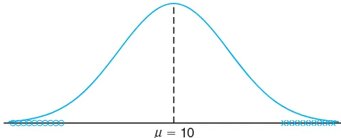
The section outlines the nature of statistical hypotheses and their role in decision-making processes across various fields, such as medicine and engineering. It emphasizes that hypotheses can only be accepted or rejected based on sample data, which leads to the development of statistical inference methodologies. The definition of a statistical hypothesis is introduced, emphasizing its reliance on sample evidence rather than absolute certainty, thus underlining the practical challenges faced when testing hypotheses.
10.2 Testing a Statistical Hypothesis
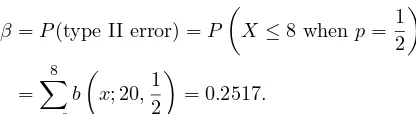
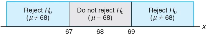
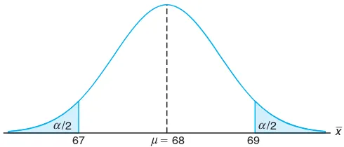
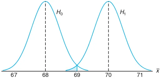
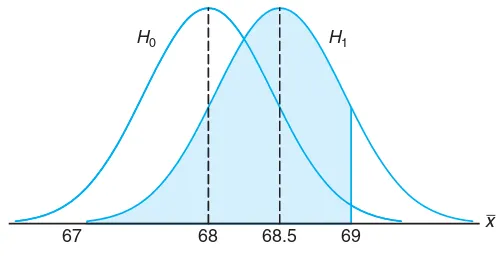
This subsection details the steps involved in testing hypotheses, including the formulation of null and alternative hypotheses. It introduces the concept of test statistics and critical values, which are essential for determining acceptance or rejection of hypotheses. The section also discusses the implications of Type I and Type II errors, enhancing the reader's understanding of the risks involved in hypothesis testing, and provides practical examples that illustrate these concepts in action.
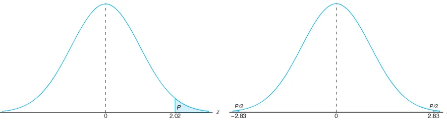
10.3 The Use of P-Values for Decision Making in Testing Hypotheses
The discussion shifts to the use of P-values as a modern approach to hypothesis testing. This section contrasts traditional fixed significance levels with the P-value method, which offers a more nuanced understanding of the evidence against the null hypothesis. The P-value is defined as the smallest significance level at which the null hypothesis can be rejected, providing a probabilistic measure that aids in decision-making. This approach is increasingly relevant in applied statistics, allowing for more flexible interpretations of test results.
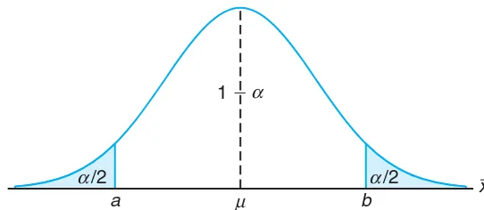
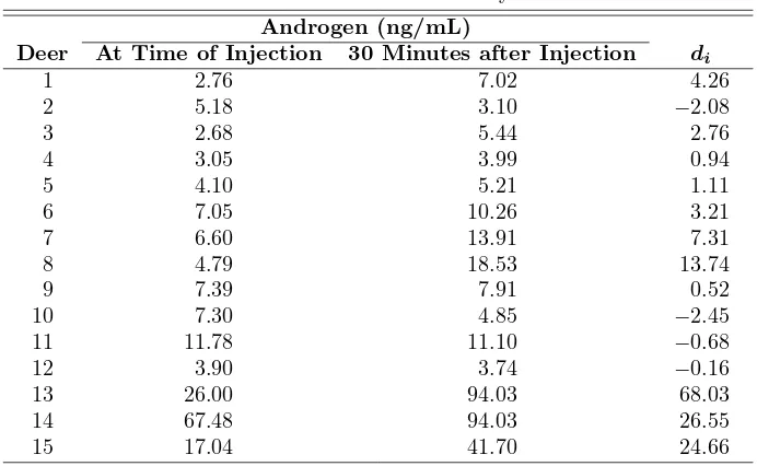
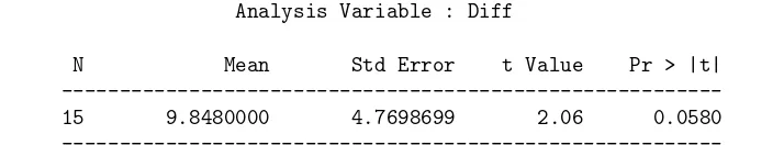
10.4 Single Sample: Tests Concerning a Single Mean
This section focuses on hypothesis testing related to a single population mean, detailing procedures for both one-tailed and two-tailed tests. The importance of understanding the relationship between hypothesis testing and confidence intervals is emphasized, as both concepts are integral to statistical inference. The section provides examples that illustrate the application of these tests in real-world scenarios, reinforcing the practical significance of hypothesis testing in engineering and scientific research.