Probability & Statistics for
Engineers & Scientists
N I N T H
E D I T I O N
Ronald E. Walpole
Roanoke College
Raymond H. Myers
Virginia Tech
Sharon L. Myers
Radford University
Keying Ye
University of Texas at San Antonio
Chapter 1
Introduction to Statistics
and Data Analysis
1.1
Overview: Statistical Inference, Samples, Populations,
and the Role of Probability
Beginning in the 1980s and continuing into the 21st century, an inordinate amount of attention has been focused on improvement of quality in American industry. Much has been said and written about the Japanese “industrial miracle,” which began in the middle of the 20th century. The Japanese were able to succeed where we and other countries had failed–namely, to create an atmosphere that allows the production of high-quality products. Much of the success of the Japanese has been attributed to the use of statistical methods and statistical thinking among management personnel.
Use of Scientific Data
The use of statistical methods in manufacturing, development of food products, computer software, energy sources, pharmaceuticals, and many other areas involves the gathering of information or scientific data. Of course, the gathering of data is nothing new. It has been done for well over a thousand years. Data have been collected, summarized, reported, and stored for perusal. However, there is a profound distinction between collection of scientific information and inferential statistics. It is the latter that has received rightful attention in recent decades.
The offspring of inferential statistics has been a large “toolbox” of statistical methods employed by statistical practitioners. These statistical methods are de-signed to contribute to the process of making scientific judgments in the face of
uncertaintyandvariation. The product density of a particular material from a manufacturing process will not always be the same. Indeed, if the process involved is a batch process rather than continuous, there will be not only variation in ma-terial density among the batches that come off the line (batch-to-batch variation), but also within-batch variation. Statistical methods are used to analyze data from a process such as this one in order to gain more sense of where in the process changes may be made to improve thequalityof the process. In this process,
ity may well be defined in relation to closeness to a target density value in harmony with what portion of the timethis closeness criterion is met. An engineer may be concerned with a specific instrument that is used to measure sulfur monoxide in the air during pollution studies. If the engineer has doubts about the effectiveness of the instrument, there are two sources of variation that must be dealt with. The first is the variation in sulfur monoxide values that are found at the same locale on the same day. The second is the variation between values observed and thetrueamount of sulfur monoxide that is in the air at the time. If either of these two sources of variation is exceedingly large (according to some standard set by the engineer), the instrument may need to be replaced. In a biomedical study of a new drug that reduces hypertension, 85% of patients experienced relief, while it is generally recognized that the current drug, or “old” drug, brings relief to 80% of pa-tients that have chronic hypertension. However, the new drug is more expensive to make and may result in certain side effects. Should the new drug be adopted? This is a problem that is encountered (often with much more complexity) frequently by pharmaceutical firms in conjunction with the FDA (Federal Drug Administration). Again, the consideration of variation needs to be taken into account. The “85%” value is based on a certain number of patients chosen for the study. Perhaps if the study were repeated with new patients the observed number of “successes” would be 75%! It is the natural variation from study to study that must be taken into account in the decision process. Clearly this variation is important, since variation from patient to patient is endemic to the problem.
Variability in Scientific Data
In the problems discussed above the statistical methods used involve dealing with variability, and in each case the variability to be studied is that encountered in scientific data. If the observed product density in the process were always the same and were always on target, there would be no need for statistical methods. If the device for measuring sulfur monoxide always gives the same value and the value is accurate (i.e., it is correct), no statistical analysis is needed. If there were no patient-to-patient variability inherent in the response to the drug (i.e., it either always brings relief or not), life would be simple for scientists in the pharmaceutical firms and FDA and no statistician would be needed in the decision process. Statistics researchers have produced an enormous number of analytical methods that allow for analysis of data from systems like those described above. This reflects the true nature of the science that we call inferential statistics, namely, using techniques that allow us to go beyond merely reporting data to drawing conclusions (or inferences) about the scientific system. Statisticians make use of fundamental laws of probability and statistical inference to draw conclusions about scientific systems. Information is gathered in the form of samples, or collections of observations. The process of sampling is introduced in Chapter 2, and the discussion continues throughout the entire book.
1.1 Overview: Statistical Inference, Samples, Populations, and the Role of Probability 3
computer boards manufactured by the firm over a specific period of time. If an improvement is made in the computer board process and a second sample of boards is collected, any conclusions drawn regarding the effectiveness of the change in pro-cess should extend to the entire population of computer boards produced under the “improved process.” In a drug experiment, a sample of patients is taken and each is given a specific drug to reduce blood pressure. The interest is focused on drawing conclusions about the population of those who suffer from hypertension.
Often, it is very important to collect scientific data in a systematic way, with planning being high on the agenda. At times the planning is, by necessity, quite limited. We often focus only on certain properties or characteristics of the items or objects in the population. Each characteristic has particular engineering or, say, biological importance to the “customer,” the scientist or engineer who seeks to learn about the population. For example, in one of the illustrations above the quality of the process had to do with the product density of the output of a process. An engineer may need to study the effect of process conditions, temperature, humidity, amount of a particular ingredient, and so on. He or she can systematically move thesefactors to whatever levels are suggested according to whatever prescription or experimental designis desired. However, a forest scientist who is interested in a study of factors that influence wood density in a certain kind of tree cannot necessarily design an experiment. This case may require anobservational study
in which data are collected in the field but factor levels can not be preselected. Both of these types of studies lend themselves to methods of statistical inference. In the former, the quality of the inferences will depend on proper planning of the experiment. In the latter, the scientist is at the mercy of what can be gathered. For example, it is sad if an agronomist is interested in studying the effect of rainfall on plant yield and the data are gathered during a drought.
The importance of statistical thinking by managers and the use of statistical inference by scientific personnel is widely acknowledged. Research scientists gain much from scientific data. Data provide understanding of scientific phenomena. Product and process engineers learn a great deal in their off-line efforts to improve the process. They also gain valuable insight by gathering production data (on-line monitoring) on a regular basis. This allows them to determine necessary modifications in order to keep the process at a desired level of quality.
There are times when a scientific practitioner wishes only to gain some sort of summary of a set of data represented in the sample. In other words, inferential statistics is not required. Rather, a set of single-number statistics or descriptive statistics is helpful. These numbers give a sense of center of the location of the data, variability in the data, and the general nature of the distribution of observations in the sample. Though no specific statistical methods leading to
The Role of Probability
In this book, Chapters 2 to 6 deal with fundamental notions of probability. A thorough grounding in these concepts allows the reader to have a better under-standing of statistical inference. Without some formalism of probability theory, the student cannot appreciate the true interpretation from data analysis through modern statistical methods. It is quite natural to study probability prior to study-ing statistical inference. Elements of probability allow us to quantify the strength or “confidence” in our conclusions. In this sense, concepts in probability form a major component that supplements statistical methods and helps us gauge the strength of the statistical inference. The discipline of probability, then, provides the transition between descriptive statistics and inferential methods. Elements of probability allow the conclusion to be put into the language that the science or engineering practitioners require. An example follows that will enable the reader to understand the notion of a P-value, which often provides the “bottom line” in the interpretation of results from the use of statistical methods.
Example 1.1: Suppose that an engineer encounters data from a manufacturing process in which 100 items are sampled and 10 are found to be defective. It is expected and antic-ipated that occasionally there will be defective items. Obviously these 100 items represent the sample. However, it has been determined that in the long run, the company can only tolerate 5% defective in the process. Now, the elements of prob-ability allow the engineer to determine how conclusive the sample information is regarding the nature of the process. In this case, the population conceptually represents all possible items from the process. Suppose we learn thatif the process is acceptable, that is, if it does produce items no more than 5% of which are de-fective, there is a probability of 0.0282 of obtaining 10 or more defective items in a random sample of 100 items from the process. This small probability suggests that the process does, indeed, have a long-run rate of defective items that exceeds 5%. In other words, under the condition of an acceptable process, the sample in-formation obtained would rarely occur. However, it did occur! Clearly, though, it would occur with a much higher probability if the process defective rate exceeded 5% by a significant amount.
From this example it becomes clear that the elements of probability aid in the translation of sample information into something conclusive or inconclusive about the scientific system. In fact, what was learned likely is alarming information to the engineer or manager. Statistical methods, which we will actually detail in Chapter 10, produced a P-value of 0.0282. The result suggests that the process
very likely is not acceptable. The concept of aP-valueis dealt with at length in succeeding chapters. The example that follows provides a second illustration.
1.1 Overview: Statistical Inference, Samples, Populations, and the Role of Probability 5
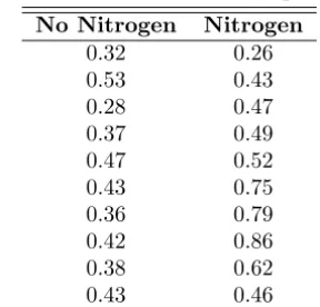
the other containing seedlings with no nitrogen. All other environmental conditions were held constant. All seedlings contained the fungusPisolithus tinctorus. More details are supplied in Chapter 9. The stem weights in grams were recorded after the end of 140 days. The data are given in Table 1.1.
Table 1.1: Data Set for Example 1.2
No Nitrogen Nitrogen
0.32 0.26
0.53 0.43
0.28 0.47
0.37 0.49
0.47 0.52
0.43 0.75
0.36 0.79
0.42 0.86
0.38 0.62
0.43 0.46
0.25 0.30 0.35 0.40 0.45 0.50 0.55 0.60 0.65 0.70 0.75 0.80 0.85 0.90
Figure 1.1: A dot plot of stem weight data.
How Do Probability and Statistical Inference Work Together?
It is important for the reader to understand the clear distinction between the discipline of probability, a science in its own right, and the discipline of inferen-tial statistics. As we have already indicated, the use or application of concepts in probability allows real-life interpretation of the results of statistical inference. As a result, it can be said that statistical inference makes use of concepts in probability. One can glean from the two examples above that the sample information is made available to the analyst and, with the aid of statistical methods and elements of probability, conclusions are drawn about some feature of the population (the pro-cess does not appear to be acceptable in Example 1.1, and nitrogen does appear to influence average stem weights in Example 1.2). Thus for a statistical problem,
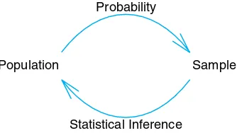
the sample along with inferential statistics allows us to draw conclu-sions about the population, with inferential statistics making clear use of elements of probability. This reasoning is inductive in nature. Now as we move into Chapter 2 and beyond, the reader will note that, unlike what we do in our two examples here, we will not focus on solving statistical problems. Many examples will be given in which no sample is involved. There will be a population clearly described with all features of the population known. Then questions of im-portance will focus on the nature of data that might hypothetically be drawn from the population. Thus, one can say that elements in probability allow us to draw conclusions about characteristics of hypothetical data taken from the population, based on known features of the population. This type of reasoning is deductivein nature. Figure 1.2 shows the fundamental relationship between probability and inferential statistics.
Population Sample Probability
Statistical Inference
Figure 1.2: Fundamental relationship between probability and inferential statistics.
Now, in the grand scheme of things, which is more important, the field of probability or the field of statistics? They are both very important and clearly are complementary. The only certainty concerning the pedagogy of the two disciplines lies in the fact that if statistics is to be taught at more than merely a “cookbook” level, then the discipline of probability must be taught first. This rule stems from the fact that nothing can be learned about a population from a sample until the analyst learns the rudiments of uncertainty in that sample. For example, consider Example 1.1. The question centers around whether or not the population, defined by the process, is no more than 5% defective. In other words, the conjecture is that
1.2 Sampling Procedures; Collection of Data 7
surface it would appear to be a refutation of the conjecture because 10 out of 100 seem to be “a bit much.” But without elements of probability, how do we know? Only through the study of material in future chapters will we learn the conditions under which the process is acceptable (5% defective). The probability of obtaining 10 or more defective items in a sample of 100 is 0.0282.
We have given two examples where the elements of probability provide a sum-mary that the scientist or engineer can use as evidence on which to build a decision. The bridge between the data and the conclusion is, of course, based on foundations of statistical inference, distribution theory, and sampling distributions discussed in future chapters.
1.2
Sampling Procedures; Collection of Data
In Section 1.1 we discussed very briefly the notion of sampling and the sampling process. While sampling appears to be a simple concept, the complexity of the questions that must be answered about the population or populations necessitates that the sampling process be very complex at times. While the notion of sampling is discussed in a technical way in Chapter 8, we shall endeavor here to give some common-sense notions of sampling. This is a natural transition to a discussion of the concept of variability.
Simple Random Sampling
The importance of proper sampling revolves around the degree of confidence with which the analyst is able to answer the questions being asked. Let us assume that only a single population exists in the problem. Recall that in Example 1.2 two populations were involved. Simple random samplingimplies that any particular sample of a specified sample size has the same chance of being selected as any other sample of the same size. The termsample sizesimply means the number of elements in the sample. Obviously, a table of random numbers can be utilized in sample selection in many instances. The virtue of simple random sampling is that it aids in the elimination of the problem of having the sample reflect a different (possibly more confined) population than the one about which inferences need to be made. For example, a sample is to be chosen to answer certain questions regarding political preferences in a certain state in the United States. The sample involves the choice of, say, 1000 families, and a survey is to be conducted. Now, suppose it turns out that random sampling is not used. Rather, all or nearly all of the 1000 families chosen live in an urban setting. It is believed that political preferences in rural areas differ from those in urban areas. In other words, the sample drawn actually confined the population and thus the inferences need to be confined to the “limited population,” and in this case confining may be undesirable. If, indeed, the inferences need to be made about the state as a whole, the sample of size 1000 described here is often referred to as abiased sample.
and a procedure called stratified random sampling involves random selection of a sample within each stratum. The purpose is to be sure that each of the strata is neither over- nor underrepresented. For example, suppose a sample survey is conducted in order to gather preliminary opinions regarding a bond referendum that is being considered in a certain city. The city is subdivided into several ethnic groups which represent natural strata. In order not to disregard or overrepresent any group, separate random samples of families could be chosen from each group.
Experimental Design
The concept of randomness or random assignment plays a huge role in the area of
experimental design, which was introduced very briefly in Section 1.1 and is an important staple in almost any area of engineering or experimental science. This will be discussed at length in Chapters 13 through 15. However, it is instructive to give a brief presentation here in the context of random sampling. A set of so-called
treatmentsortreatment combinationsbecomes the populations to be studied or compared in some sense. An example is the nitrogen versus no-nitrogen treat-ments in Example 1.2. Another simple example would be “placebo” versus “active drug,” or in a corrosion fatigue study we might have treatment combinations that involve specimens that are coated or uncoated as well as conditions of low or high humidity to which the specimens are exposed. In fact, there are four treatment or factor combinations (i.e., 4 populations), and many scientific questions may be asked and answered through statistical and inferential methods. Consider first the situation in Example 1.2. There are 20 diseased seedlings involved in the exper-iment. It is easy to see from the data themselves that the seedlings are different from each other. Within the nitrogen group (or the no-nitrogen group) there is considerable variability in the stem weights. This variability is due to what is generally called the experimental unit. This is a very important concept in in-ferential statistics, in fact one whose description will not end in this chapter. The nature of the variability is very important. If it is too large, stemming from a condition of excessive nonhomogeneity in experimental units, the variability will “wash out” any detectable difference between the two populations. Recall that in this case that did not occur.
1.2 Sampling Procedures; Collection of Data 9
Why Assign Experimental Units Randomly?
What is the possible negative impact of not randomly assigning experimental units to the treatments or treatment combinations? This is seen most clearly in the case of the drug study. Among the characteristics of the patients that produce variability in the results are age, gender, and weight. Suppose merely by chance the placebo group contains a sample of people that are predominately heavier than those in the treatment group. Perhaps heavier individuals have a tendency to have a higher blood pressure. This clearly biases the result, and indeed, any result obtained through the application of statistical inference may have little to do with the drug and more to do with differences in weights among the two samples of patients.
We should emphasize the attachment of importance to the term variability. Excessive variability among experimental units “camouflages” scientific findings. In future sections, we attempt to characterize and quantify measures of variability. In sections that follow, we introduce and discuss specific quantities that can be computed in samples; the quantities give a sense of the nature of the sample with respect to center of location of the data and variability in the data. A discussion of several of these single-number measures serves to provide a preview of what statistical information will be important components of the statistical methods that are used in future chapters. These measures that help characterize the nature of the data set fall into the category ofdescriptive statistics. This material is a prelude to a brief presentation of pictorial and graphical methods that go even further in characterization of the data set. The reader should understand that the statistical methods illustrated here will be used throughout the text. In order to offer the reader a clearer picture of what is involved in experimental design studies, we offer Example 1.3.
Example 1.3: A corrosion study was made in order to determine whether coating an aluminum metal with a corrosion retardation substance reduced the amount of corrosion. The coating is a protectant that is advertised to minimize fatigue damage in this type of material. Also of interest is the influence of humidity on the amount of corrosion. A corrosion measurement can be expressed in thousands of cycles to failure. Two levels of coating, no coating and chemical corrosion coating, were used. In addition, the two relative humidity levels are 20% relative humidity and 80% relative humidity.
The experiment involves four treatment combinations that are listed in the table that follows. There are eight experimental units used, and they are aluminum specimens prepared; two are assigned randomly to each of the four treatment combinations. The data are presented in Table 1.2.
The corrosion data are averages of two specimens. A plot of the averages is pictured in Figure 1.3. A relatively large value of cycles to failure represents a small amount of corrosion. As one might expect, an increase in humidity appears to make the corrosion worse. The use of the chemical corrosion coating procedure appears to reduce corrosion.
Table 1.2: Data for Example 1.3
Average Corrosion in Coating Humidity Thousands of Cycles to Failure
Uncoated 20% 975
80% 350
Chemical Corrosion 20% 1750
80% 1550
0 1000 2000
0 20% 80%
Humidity
Average Corrosion
Uncoated Chemical Corrosion Coating
Figure 1.3: Corrosion results for Example 1.3.
conditions representing the four treatment combinations are four separate popula-tions and that the two corrosion values observed for each population are important pieces of information. The importance of the average in capturing and summariz-ing certain features in the population will be highlighted in Section 1.3. While we might draw conclusions about the role of humidity and the impact of coating the specimens from the figure, we cannot truly evaluate the results from an analyti-cal point of view without taking into account the variability around the average. Again, as we indicated earlier, if the two corrosion values for each treatment com-bination are close together, the picture in Figure 1.3 may be an accurate depiction. But if each corrosion value in the figure is an average of two values that are widely dispersed, then this variability may, indeed, truly “wash away” any information that appears to come through when one observes averages only. The foregoing example illustrates these concepts:
(1) random assignment of treatment combinations (coating, humidity) to experi-mental units (specimens)
(2) the use of sample averages (average corrosion values) in summarizing sample information
1.3 Measures of Location: The Sample Mean and Median 11
This example suggests the need for what follows in Sections 1.3 and 1.4, namely, descriptive statistics that indicate measures of center of location in a set of data, and those that measure variability.
1.3
Measures of Location: The Sample Mean and Median
Measures of location are designed to provide the analyst with some quantitative values of where the center, or some other location, of data is located. In Example 1.2, it appears as if the center of the nitrogen sample clearly exceeds that of the no-nitrogen sample. One obvious and very useful measure is thesample mean. The mean is simply a numerical average.
Definition 1.1: Suppose that the observations in a sample arex1, x2, . . . , xn. Thesample mean, denoted by ¯x, is
¯
x=
n
i=1
xi
n =
x1+x2+· · ·+xn
n .
There are other measures of central tendency that are discussed in detail in future chapters. One important measure is thesample median. The purpose of the sample median is to reflect the central tendency of the sample in such a way that it is uninfluenced by extreme values or outliers.
Definition 1.2: Given that the observations in a sample arex1, x2, . . . , xn, arranged inincreasing
orderof magnitude, the sample median is
˜
x=
x(n+1)/2, ifnis odd, 1
2(xn/2+xn/2+1), ifnis even.
As an example, suppose the data set is the following: 1.7, 2.2, 3.9, 3.11, and 14.7. The sample mean and median are, respectively,
¯
x= 5.12, x˜= 3.9.
Clearly, the mean is influenced considerably by the presence of the extreme obser-vation, 14.7, whereas the median places emphasis on the true “center” of the data set. In the case of the two-sample data set of Example 1.2, the two measures of central tendency for the individual samples are
¯
x(no nitrogen) = 0.399 gram,
˜
x(no nitrogen) = 0.38 + 0.42
2 = 0.400 gram, ¯
x(nitrogen) = 0.565 gram,
˜
x(nitrogen) = 0.49 + 0.52
2 = 0.505 gram.
is the centroid of the data in a sample. In a sense, it is the point at which a fulcrum can be placed to balance a system of “weights” which are the locations of the individual data. This is shown in Figure 1.4 with regard to the with-nitrogen sample.
0.25 0.30 0.35 0.40 0.45 0.50 0.55 0.60 0.65 0.70 0.75 0.80 0.85 0.90 x ⫽ 0.565
Figure 1.4: Sample mean as a centroid of the with-nitrogen stem weight.
In future chapters, the basis for the computation of ¯xis that of an estimate
of thepopulation mean. As we indicated earlier, the purpose of statistical infer-ence is to draw conclusions about population characteristics or parameters and
estimation is a very important feature of statistical inference.
The median and mean can be quite different from each other. Note, however, that in the case of the stem weight data the sample mean value for no-nitrogen is quite similar to the median value.
Other Measures of Locations
There are several other methods of quantifying the center of location of the data in the sample. We will not deal with them at this point. For the most part, alternatives to the sample mean are designed to produce values that represent compromises between the mean and the median. Rarely do we make use of these other measures. However, it is instructive to discuss one class of estimators, namely the class of trimmed means. A trimmed mean is computed by “trimming away” a certain percent of both the largest and the smallest set of values. For example, the 10% trimmed mean is found by eliminating the largest 10% and smallest 10% and computing the average of the remaining values. For example, in the case of the stem weight data, we would eliminate the largest and smallest since the sample size is 10 for each sample. So for the without-nitrogen group the 10% trimmed mean is given by
¯
xtr(10) =0.32 + 0.37 + 0.47 + 0.43 + 0.36 + 0.42 + 0.38 + 0.43
8 = 0.39750,
and for the 10% trimmed mean for the with-nitrogen group we have
¯
xtr(10) =0.43 + 0.47 + 0.49 + 0.52 + 0.75 + 0.79 + 0.62 + 0.46
8 = 0.56625.
/ /
Exercises 13
Exercises
1.1 The following measurements were recorded for the drying time, in hours, of a certain brand of latex paint.
3.4 2.5 4.8 2.9 3.6 2.8 3.3 5.6 3.7 2.8 4.4 4.0 5.2 3.0 4.8
Assume that the measurements are a simple random sample.
(a) What is the sample size for the above sample? (b) Calculate the sample mean for these data. (c) Calculate the sample median.
(d) Plot the data by way of a dot plot.
(e) Compute the 20% trimmed mean for the above data set.
(f) Is the sample mean for these data more or less de-scriptive as a center of location than the trimmed mean?
1.2 According to the journal Chemical Engineering, an important property of a fiber is its water ab-sorbency. A random sample of 20 pieces of cotton fiber was taken and the absorbency on each piece was mea-sured. The following are the absorbency values:
18.71 21.41 20.72 21.81 19.29 22.43 20.17 23.71 19.44 20.50 18.92 20.33 23.00 22.85 19.25 21.77 22.11 19.77 18.04 21.12
(a) Calculate the sample mean and median for the above sample values.
(b) Compute the 10% trimmed mean. (c) Do a dot plot of the absorbency data.
(d) Using only the values of the mean, median, and trimmed mean, do you have evidence of outliers in the data?
1.3 A certain polymer is used for evacuation systems for aircraft. It is important that the polymer be re-sistant to the aging process. Twenty specimens of the polymer were used in an experiment. Ten were as-signed randomly to be exposed to an accelerated batch aging process that involved exposure to high tempera-tures for 10 days. Measurements of tensile strength of the specimens were made, and the following data were recorded on tensile strength in psi:
No aging: 227 222 218 217 225 218 216 229 228 221 Aging: 219 214 215 211 209 218 203 204 201 205 (a) Do a dot plot of the data.
(b) From your plot, does it appear as if the aging pro-cess has had an effect on the tensile strength of this
polymer? Explain.
(c) Calculate the sample mean tensile strength of the two samples.
(d) Calculate the median for both. Discuss the simi-larity or lack of simisimi-larity between the mean and median of each group.
1.4 In a study conducted by the Department of Me-chanical Engineering at Virginia Tech, the steel rods supplied by two different companies were compared. Ten sample springs were made out of the steel rods supplied by each company, and a measure of flexibility was recorded for each. The data are as follows:
Company A: 9.3 8.8 6.8 8.7 8.5 6.7 8.0 6.5 9.2 7.0 Company B: 11.0 9.8 9.9 10.2 10.1 9.7 11.0 11.1 10.2 9.6 (a) Calculate the sample mean and median for the data
for the two companies.
(b) Plot the data for the two companies on the same line and give your impression regarding any appar-ent differences between the two companies.
1.5 Twenty adult males between the ages of 30 and 40 participated in a study to evaluate the effect of a specific health regimen involving diet and exercise on the blood cholesterol. Ten were randomly selected to be a control group, and ten others were assigned to take part in the regimen as the treatment group for a period of 6 months. The following data show the re-duction in cholesterol experienced for the time period for the 20 subjects:
(b) Compute the mean, median, and 10% trimmed mean for both groups.
(c) Explain why the difference in means suggests one conclusion about the effect of the regimen, while the difference in medians or trimmed means sug-gests a different conclusion.
1.6 The tensile strength of silicone rubber is thought to be a function of curing temperature. A study was carried out in which samples of 12 specimens of the rub-ber were prepared using curing temperatures of 20◦C
and 45◦C. The data below show the tensile strength
20◦C: 2.07 2.14 2.22 2.03 2.21 2.03
2.05 2.18 2.09 2.14 2.11 2.02 45◦C: 2.52 2.15 2.49 2.03 2.37 2.05
1.99 2.42 2.08 2.42 2.29 2.01
(a) Show a dot plot of the data with both low and high temperature tensile strength values.
(b) Compute sample mean tensile strength for both samples.
(c) Does it appear as if curing temperature has an influence on tensile strength, based on the plot? Comment further.
(d) Does anything else appear to be influenced by an increase in curing temperature? Explain.
1.4
Measures of Variability
Sample variability plays an important role in data analysis. Process and product variability is a fact of life in engineering and scientific systems: The control or reduction of process variability is often a source of major difficulty. More and more process engineers and managers are learning that product quality and, as a result, profits derived from manufactured products are very much a function of process variability. As a result, much of Chapters 9 through 15 deals with data analysis and modeling procedures in which sample variability plays a major role. Even in small data analysis problems, the success of a particular statistical method may depend on the magnitude of the variability among the observations in the sample. Measures of location in a sample do not provide a proper summary of the nature of a data set. For instance, in Example 1.2 we cannot conclude that the use of nitrogen enhances growth without taking sample variability into account.
While the details of the analysis of this type of data set are deferred to Chap-ter 9, it should be clear from Figure 1.1 that variability among the no-nitrogen observations and variability among the nitrogen observations are certainly of some consequence. In fact, it appears that the variability within the nitrogen sample is larger than that of the no-nitrogen sample. Perhaps there is something about the inclusion of nitrogen that not only increases the stem height (¯xof 0.565 gram compared to an ¯xof 0.399 gram for the no-nitrogen sample) but also increases the variability in stem height (i.e., renders the stem height more inconsistent).
As another example, contrast the two data sets below. Each contains two samples and the difference in the means is roughly the same for the two samples, but data set B seems to provide a much sharper contrast between the two populations from which the samples were taken. If the purpose of such an experiment is to detect differences between the two populations, the task is accomplished in the case of data set B. However, in data set A the large variability withinthe two samples creates difficulty. In fact, it is not clear that there is a distinctionbetweenthe two populations.
Data set A: X X X X X X 0 X X 0 0 X X X 0 0 0 0 0 0 0 0
Data set B: X X X X X X X X X X X 0 0 0 0 0 0 0 0 0 0 0
xX x0
1.4 Measures of Variability 15
Sample Range and Sample Standard Deviation
Just as there are many measures of central tendency or location, there are many measures of spread or variability. Perhaps the simplest one is the sample range Xmax−Xmin. The range can be very useful and is discussed at length in Chapter
17 on statistical quality control. The sample measure of spread that is used most often is the sample standard deviation. We again let x1, x2, . . . , xn denote
sample values.
Definition 1.3: Thesample variance, denoted bys2, is given by
s2=
n
i=1
(xi−x¯)2
n−1 .
Thesample standard deviation, denoted bys, is the positive square root of
s2, that is,
s=√s2.
It should be clear to the reader that the sample standard deviation is, in fact, a measure of variability. Large variability in a data set produces relatively large values of (x−x¯)2 and thus a large sample variance. The quantity n−1 is often called thedegrees of freedom associated with the varianceestimate. In this simple example, the degrees of freedom depict the number of independent pieces of information available for computing variability. For example, suppose that we wish to compute the sample variance and standard deviation of the data set (5, 17, 6, 4). The sample average is ¯x= 8. The computation of the variance involves
(5−8)2+ (17−8)2+ (6−8)2+ (4−8)2= (−3)2+ 92+ (−2)2+ (−4)2.
The quantities inside parentheses sum to zero. In general,
n
i=1
(xi−¯x) = 0 (see Exercise 1.16 on page 31). Then the computation of a sample variance does not involvenindependent squared deviationsfrom the mean ¯x. In fact, since the last value of x−x¯ is determined by the initial n−1 of them, we say that these are n−1 “pieces of information” that produce s2. Thus, there are n−1 degrees of freedom rather thanndegrees of freedom for computing a sample variance.
Example 1.4: In an example discussed extensively in Chapter 10, an engineer is interested in testing the “bias” in a pH meter. Data are collected on the meter by measuring the pH of a neutral substance (pH = 7.0). A sample of size 10 is taken, with results given by
7.07 7.00 7.10 6.97 7.00 7.03 7.01 7.01 6.98 7.08.
The sample mean ¯xis given by
¯
x= 7.07 + 7.00 + 7.10 +· · ·+ 7.08
The sample variance s2is given by
s2= 1
9[(7.07−7.025)
2+ (7.00
−7.025)2+ (7.10−7.025)2
+· · ·+ (7.08−7.025)2] = 0.001939.
As a result, the sample standard deviation is given by
s=√0.001939 = 0.044.
So the sample standard deviation is 0.0440 withn−1 = 9 degrees of freedom.
Units for Standard Deviation and Variance
It should be apparent from Definition 1.3 that the variance is a measure of the average squared deviation from the mean ¯x. We use the term average squared deviationeven though the definition makes use of a division by degrees of freedom
n−1 rather than n. Of course, if n is large, the difference in the denominator is inconsequential. As a result, the sample variance possesses units that are the square of the units in the observed data whereas the sample standard deviation is found in linear units. As an example, consider the data of Example 1.2. The stem weights are measured in grams. As a result, the sample standard deviations are in grams and the variances are measured in grams2. In fact, the individual standard deviations are 0.0728 gram for the no-nitrogen case and 0.1867 gram for the nitrogen group. Note that the standard deviation does indicate considerably larger variability in the nitrogen sample. This condition was displayed in Figure 1.1.
Which Variability Measure Is More Important?
As we indicated earlier, the sample range has applications in the area of statistical quality control. It may appear to the reader that the use of both the sample variance and the sample standard deviation is redundant. Both measures reflect the same concept in measuring variability, but the sample standard deviation measures variability in linear units whereas the sample variance is measured in squared units. Both play huge roles in the use of statistical methods. Much of what is accomplished in the context of statistical inference involves drawing conclusions about characteristics of populations. Among these characteristics are constants which are called population parameters. Two important parameters are the
1.5 Discrete and Continuous Data 17
Exercises
1.7 Consider the drying time data for Exercise 1.1 on page 13. Compute the sample variance and sample standard deviation.
1.8 Compute the sample variance and standard devi-ation for the water absorbency data of Exercise 1.2 on page 13.
1.9 Exercise 1.3 on page 13 showed tensile strength data for two samples, one in which specimens were ex-posed to an aging process and one in which there was no aging of the specimens.
(a) Calculate the sample variance as well as standard deviation in tensile strength for both samples. (b) Does there appear to be any evidence that aging
affects the variability in tensile strength? (See also the plot for Exercise 1.3 on page 13.)
1.10 For the data of Exercise 1.4 on page 13, com-pute both the mean and the variance in “flexibility” for both company A and company B. Does there ap-pear to be a difference in flexibility between company A and company B?
1.11 Consider the data in Exercise 1.5 on page 13. Compute the sample variance and the sample standard deviation for both control and treatment groups.
1.12 For Exercise 1.6 on page 13, compute the sample standard deviation in tensile strength for the samples separately for the two temperatures. Does it appear as if an increase in temperature influences the variability in tensile strength? Explain.
1.5
Discrete and Continuous Data
Statistical inference through the analysis of observational studies or designed ex-periments is used in many scientific areas. The data gathered may be discrete
or continuous, depending on the area of application. For example, a chemical engineer may be interested in conducting an experiment that will lead to condi-tions where yield is maximized. Here, of course, the yield may be in percent or grams/pound, measured on a continuum. On the other hand, a toxicologist con-ducting a combination drug experiment may encounter data that are binary in nature (i.e., the patient either responds or does not).
Great distinctions are made between discrete and continuous data in the prob-ability theory that allow us to draw statistical inferences. Often applications of statistical inference are found when the data are count data. For example, an en-gineer may be interested in studying the number of radioactive particles passing through a counter in, say, 1 millisecond. Personnel responsible for the efficiency of a port facility may be interested in the properties of the number of oil tankers arriving each day at a certain port city. In Chapter 5, several distinct scenarios, leading to different ways of handling data, are discussed for situations with count data.
the drug was a success and 1−0.4 = 0.6 is the sample proportion for which the drug was not successful. Actually the basic numerical measurement for binary data is generally denoted by either 0 or 1. For example, in our medical example, a successful result is denoted by a 1 and a nonsuccess a 0. As a result, the sample proportion is actually a sample mean of the ones and zeros. For the successful category,
x1+x2+· · ·+x50
50 =
1 + 1 + 0 +· · ·+ 0 + 1
50 =
20 50 = 0.4.
What Kinds of Problems Are Solved in Binary Data Situations?
The kinds of problems facing scientists and engineers dealing in binary data are not a great deal unlike those seen where continuous measurements are of interest. However, different techniques are used since the statistical properties of sample proportions are quite different from those of the sample means that result from averages taken from continuous populations. Consider the example data in Ex-ercise 1.6 on page 13. The statistical problem underlying this illustration focuses on whether an intervention, say, an increase in curing temperature, will alter the population mean tensile strength associated with the silicone rubber process. On the other hand, in a quality control area, suppose an automobile tire manufacturer reports that a shipment of 5000 tires selected randomly from the process results in 100 of them showing blemishes. Here the sample proportion is 5000100 = 0.02. Following a change in the process designed to reduce blemishes, a second sample of 5000 is taken and 90 tires are blemished. The sample proportion has been reduced to 90
5000 = 0.018. The question arises, “Is the decrease in the sample proportion from 0.02 to 0.018 substantial enough to suggest a real improvement in the pop-ulation proportion?” Both of these illustrations require the use of the statistical properties of sample averages—one from samples from a continuous population, and the other from samples from a discrete (binary) population. In both cases, the sample mean is an estimate of a population parameter, a population mean in the first illustration (i.e., mean tensile strength), and a population proportion in the second case (i.e., proportion of blemished tires in the population). So here we have sample estimates used to draw scientific conclusions regarding population parameters. As we indicated in Section 1.3, this is the general theme in many practical problems using statistical inference.
1.6
Statistical Modeling, Scientific Inspection, and Graphical
Diagnostics
Often the end result of a statistical analysis is the estimation of parameters of a
postulated model. This is natural for scientists and engineers since they often deal in modeling. A statistical model is not deterministic but, rather, must entail some probabilistic aspects. A model form is often the foundation of assumptions
1.6 Statistical Modeling, Scientific Inspection, and Graphical Diagnostics 19
the data, for example, that the two samples come from normal or Gaussian distributions. See Chapter 6 for a discussion of the normal distribution.
Obviously, the user of statistical methods cannot generate sufficient informa-tion or experimental data to characterize the populainforma-tion totally. But sets of data are often used to learn about certain properties of the population. Scientists and engineers are accustomed to dealing with data sets. The importance of character-izing or summarizingthe nature of collections of data should be obvious. Often a summary of a collection of data via a graphical display can provide insight regard-ing the system from which the data were taken. For instance, in Sections 1.1 and 1.3, we have shown dot plots.
In this section, the role of sampling and the display of data for enhancement of
statistical inferenceis explored in detail. We merely introduce some simple but often effective displays that complement the study of statistical populations.
Scatter Plot
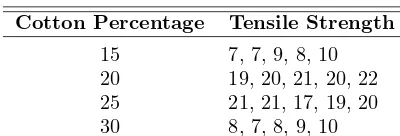
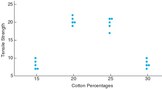
At times the model postulated may take on a somewhat complicated form. Con-sider, for example, a textile manufacturer who designs an experiment where cloth specimen that contain various percentages of cotton are produced. Consider the data in Table 1.3.
Table 1.3: Tensile Strength
Cotton Percentage Tensile Strength
15 7, 7, 9, 8, 10 20 19, 20, 21, 20, 22 25 21, 21, 17, 19, 20 30 8, 7, 8, 9, 10
around a different type of model, one that postulates a type of structure relating the population mean tensile strength to the cotton concentration. In other words, a model may be written
μt,c=β0+β1C+β2C2,
where μt,c is the population mean tensile strength, which varies with the amount
of cotton in the productC. The implication of this model is that for a fixed cotton level, there is a population of tensile strength measurements and the population mean is μt,c. This type of model, called a regression model, is discussed in
Chapters 11 and 12. The functional form is chosen by the scientist. At times the data analysis may suggest that the model be changed. Then the data analyst “entertains” a model that may be altered after some analysis is done. The use of an empirical model is accompanied by estimation theory, whereβ0,β1, and
β2 are estimated by the data. Further, statistical inference can then be used to determine model adequacy.
5 10 15 20 25
15 20 25 30
Tensile Strength
Cotton Percentages
Figure 1.5: Scatter plot of tensile strength and cotton percentages.
1.6 Statistical Modeling, Scientific Inspection, and Graphical Diagnostics 21
Stem-and-Leaf Plot
Statistical data, generated in large masses, can be very useful for studying the behavior of the distribution if presented in a combined tabular and graphic display called astem-and-leaf plot.
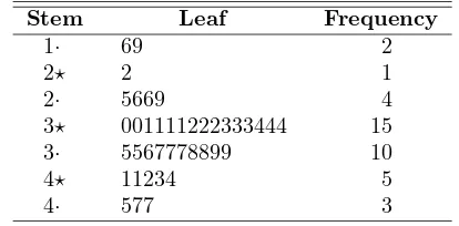
To illustrate the construction of a stem-and-leaf plot, consider the data of Table 1.4, which specifies the “life” of 40 similar car batteries recorded to the nearest tenth of a year. The batteries are guaranteed to last 3 years. First, split each observation into two parts consisting of a stem and a leaf such that the stem represents the digit preceding the decimal and the leaf corresponds to the decimal part of the number. In other words, for the number 3.7, the digit 3 is designated the stem and the digit 7 is the leaf. The four stems 1, 2, 3, and 4 for our data are listed vertically on the left side in Table 1.5; the leaves are recorded on the right side opposite the appropriate stem value. Thus, the leaf 6 of the number 1.6 is recorded opposite the stem 1; the leaf 5 of the number 2.5 is recorded opposite the stem 2; and so forth. The number of leaves recorded opposite each stem is summarized under the frequency column.
Table 1.4: Car Battery Life 2.2 4.1 3.5 4.5 3.2 3.7 3.0 2.6 3.4 1.6 3.1 3.3 3.8 3.1 4.7 3.7 2.5 4.3 3.4 3.6 2.9 3.3 3.9 3.1 3.3 3.1 3.7 4.4 3.2 4.1 1.9 3.4 4.7 3.8 3.2 2.6 3.9 3.0 4.2 3.5
Table 1.5: Stem-and-Leaf Plot of Battery Life
Stem Leaf Frequency
1 2 3 4
69 25669
0011112223334445567778899 11234577
2 5 25 8
The stem-and-leaf plot of Table 1.5 contains only four stems and consequently does not provide an adequate picture of the distribution. To remedy this problem, we need to increase the number of stems in our plot. One simple way to accomplish this is to write each stem value twice and then record the leaves 0, 1, 2, 3, and 4 opposite the appropriate stem value where it appears for the first time, and the leaves 5, 6, 7, 8, and 9 opposite this same stem value where it appears for the second time. This modified double-stem-and-leaf plot is illustrated in Table 1.6, where the stems corresponding to leaves 0 through 4 have been coded by the symbol ⋆ and the stems corresponding to leaves 5 through 9 by the symbol·.
the data consist of numbers from 1 to 21 representing the number of people in a cafeteria line on 40 randomly selected workdays and we choose a double-stem-and-leaf plot, the stems will be 0⋆, 0·, 1⋆, 1·, and 2⋆ so that the smallest observation 1 has stem 0⋆ and leaf 1, the number 18 has stem 1· and leaf 8, and the largest observation 21 has stem 2⋆ and leaf 1. On the other hand, if the data consist of numbers from $18,800 to $19,600 representing the best possible deals on 100 new automobiles from a certain dealership and we choose a single-stem-and-leaf plot, the stems will be 188, 189, 190, . . ., 196 and the leaves will now each contain two digits. A car that sold for $19,385 would have a stem value of 193 and the two-digit leaf 85. Multiple-digit leaves belonging to the same stem are usually separated by commas in the stem-and-leaf plot. Decimal points in the data are generally ignored when all the digits to the right of the decimal represent the leaf. Such was the case in Tables 1.5 and 1.6. However, if the data consist of numbers ranging from 21.8 to 74.9, we might choose the digits 2, 3, 4, 5, 6, and 7 as our stems so that a number such as 48.3 would have a stem value of 4 and a leaf of 8.3.
Table 1.6: Double-Stem-and-Leaf Plot of Battery Life
Stem Leaf Frequency
The stem-and-leaf plot represents an effective way to summarize data. Another way is through the use of the frequency distribution, where the data, grouped into different classes or intervals, can be constructed by counting the leaves be-longing to each stem and noting that each stem defines a class interval. In Table 1.5, the stem 1 with 2 leaves defines the interval 1.0–1.9 containing 2 observations; the stem 2 with 5 leaves defines the interval 2.0–2.9 containing 5 observations; the stem 3 with 25 leaves defines the interval 3.0–3.9 with 25 observations; and the stem 4 with 8 leaves defines the interval 4.0–4.9 containing 8 observations. For the double-stem-and-leaf plot of Table 1.6, the stems define the seven class intervals 1.5–1.9, 2.0–2.4, 2.5–2.9, 3.0–3.4, 3.5–3.9, 4.0–4.4, and 4.5–4.9 with frequencies 2, 1, 4, 15, 10, 5, and 3, respectively.
Histogram
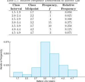
Dividing each class frequency by the total number of observations, we obtain the proportion of the set of observations in each of the classes. A table listing relative frequencies is called a relative frequency distribution. The relative frequency distribution for the data of Table 1.4, showing the midpoint of each class interval, is given in Table 1.7.
1.6 Statistical Modeling, Scientific Inspection, and Graphical Diagnostics 23
Table 1.7: Relative Frequency Distribution of Battery Life
Class Class Frequency, Relative
Interval Midpoint f Frequency
1.5–1.9 1.7 2 0.050
2.0–2.4 2.2 1 0.025
2.5–2.9 2.7 4 0.100
3.0–3.4 3.2 15 0.375
3.5–3.9 3.7 10 0.250
4.0–4.4 4.2 5 0.125
4.5–4.9 4.7 3 0.075
0.375
0.250
0.125
1.7 2.2 2.7 3.2 3.7 4.2 4.7
Relativ
e Frequencty
Battery Life (years)
Figure 1.6: Relative frequency histogram.
corresponding relative frequency, we construct arelative frequency histogram
(Figure 1.6).
Many continuous frequency distributions can be represented graphically by the characteristic bell-shaped curve of Figure 1.7. Graphical tools such as what we see in Figures 1.6 and 1.7 aid in the characterization of the nature of the population. In Chapters 5 and 6 we discuss a property of the population called itsdistribution. While a more rigorous definition of a distribution or probability distribution
will be given later in the text, at this point one can view it as what would be seen in Figure 1.7 in the limit as the size of the sample becomes larger.
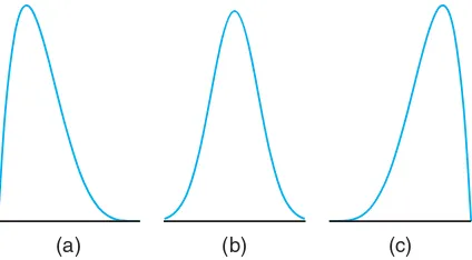
A distribution is said to besymmetricif it can be folded along a vertical axis so that the two sides coincide. A distribution that lacks symmetry with respect to a vertical axis is said to be skewed. The distribution illustrated in Figure 1.8(a) is said to be skewed to the right since it has a long right tail and a much shorter left tail. In Figure 1.8(b) we see that the distribution is symmetric, while in Figure 1.8(c) it is skewed to the left.
0
f(x)
Battery Life (years)
1 2 3 4 5 6
Figure 1.7: Estimating frequency distribution.
(a) (b) (c)
Figure 1.8: Skewness of data.
to construct a relative frequency histogram.
Box-and-Whisker Plot or Box Plot
Another display that is helpful for reflecting properties of a sample is the box-and-whisker plot. This plot encloses theinterquartile rangeof the data in a box that has the median displayed within. The interquartile range has as its extremes the 75th percentile (upper quartile) and the 25th percentile (lower quartile). In addition to the box, “whiskers” extend, showing extreme observations in the sam-ple. For reasonably large samples, the display shows center of location, variability, and the degree of asymmetry.
1.6 Statistical Modeling, Scientific Inspection, and Graphical Diagnostics 25
The visual information in the box-and-whisker plot or box plot is not intended to be a formal test for outliers. Rather, it is viewed as a diagnostic tool. While the determination of which observations are outliers varies with the type of software that is used, one common procedure is to use a multiple of the interquartile range. For example, if the distance from the box exceeds 1.5 times the interquartile range (in either direction), the observation may be labeled an outlier.
Example 1.5: Nicotine content was measured in a random sample of 40 cigarettes. The data are displayed in Table 1.8.
Table 1.8: Nicotine Data for Example 1.5
1.09 1.92 2.31 1.79 2.28 1.74 1.47 1.97 0.85 1.24 1.58 2.03 1.70 2.17 2.55 2.11 1.86 1.90 1.68 1.51 1.64 0.72 1.69 1.85 1.82 1.79 2.46 1.88 2.08 1.67 1.37 1.93 1.40 1.64 2.09 1.75 1.63 2.37 1.75 1.69
1.0 1.5 2.0 2.5 Nicotine
Figure 1.9: Box-and-whisker plot for Example 1.5.
Figure 1.9 shows the box-and-whisker plot of the data, depicting the observa-tions 0.72 and 0.85 as mild outliers in the lower tail, whereas the observation 2.55 is a mild outlier in the upper tail. In this example, the interquartile range is 0.365, and 1.5 times the interquartile range is 0.5475. Figure 1.10, on the other hand, provides a stem-and-leaf plot.
The decimal point is 1 digit(s) to the left of the | 7 | 2
8 | 5 9 | 10 | 9 11 | 12 | 4 13 | 7 14 | 07 15 | 18 16 | 3447899 17 | 045599 18 | 2568 19 | 0237 20 | 389 21 | 17 22 | 8 23 | 17 24 | 6 25 | 5
Figure 1.10: Stem-and-leaf plot for the nicotine data.
Table 1.9: Data for Example 1.6
Sample Measurements Sample Measurements
1 29 36 39 34 34 16 35 30 35 29 37 2 29 29 28 32 31 17 40 31 38 35 31 3 34 34 39 38 37 18 35 36 30 33 32 4 35 37 33 38 41 19 35 34 35 30 36 5 30 29 31 38 29 20 35 35 31 38 36 6 34 31 37 39 36 21 32 36 36 32 36 7 30 35 33 40 36 22 36 37 32 34 34 8 28 28 31 34 30 23 29 34 33 37 35 9 32 36 38 38 35 24 36 36 35 37 37 10 35 30 37 35 31 25 36 30 35 33 31 11 35 30 35 38 35 26 35 30 29 38 35 12 38 34 35 35 31 27 35 36 30 34 36 13 34 35 33 30 34 28 35 30 36 29 35 14 40 35 34 33 35 29 38 36 35 31 31 15 34 35 38 35 30 30 30 34 40 28 30
There are additional ways that box-and-whisker plots and other graphical dis-plays can aid the analyst. Multiple samples can be compared graphically. Plots of data can suggest relationships between variables. Graphs can aid in the detection of anomalies or outlying observations in samples.
1.7 General Types of Statistical Studies 27
28 30 32 34 36 38 40
Paint
Figure 1.11: Box-and-whisker plot for thickness of paint can “ears.”
Other Distinguishing Features of a Sample
There are features of the distribution or sample other than measures of center of location and variability that further define its nature. For example, while the median divides the data (or distribution) into two parts, there are other measures that divide parts or pieces of the distribution that can be very useful. Separation is made into four parts by quartiles, with the third quartile separating the upper quarter of the data from the rest, the second quartile being the median, and the first quartile separating the lower quarter of the data from the rest. The distribution can be even more finely divided by computing percentiles of the distribution. These quantities give the analyst a sense of the so-called tails of the distribution (i.e., values that are relatively extreme, either small or large). For example, the 95th percentile separates the highest 5% from the bottom 95%. Similar definitions prevail for extremes on the lower side or lower tail of the distribution. The 1st percentile separates the bottom 1% from the rest of the distribution. The concept of percentiles will play a major role in much that will be covered in future chapters.
1.7
General Types of Statistical Studies: Designed
Experiment, Observational Study, and Retrospective Study
interest to learn about some characteristic or measurement (level of corrosion) that results from these conditions. Statistical methods that make use of measures of central tendency in the corrosion measure, as well as measures of variability, are employed. As the reader will observe later in the text, these methods often lead to a statistical model like that discussed in Section 1.6. In this case, the model may be used to estimate (or predict) the corrosion measure as a function of humidity and the type of coating employed. Again, in developing this kind of model, descriptive statistics that highlight central tendency and variability become very useful.
The information supplied in Example 1.3 illustrates nicely the types of engi-neering questions asked and answered by the use of statistical methods that are employed through a designed experiment and presented in this text. They are
(i) What is the nature of the impact of relative humidity on the corrosion of the aluminum alloy within the range of relative humidity in this experiment? (ii) Does the chemical corrosion coating reduce corrosion levels and can the effect
be quantified in some fashion?
(iii) Is thereinteractionbetween coating type and relative humidity that impacts their influence on corrosion of the alloy? If so, what is its interpretation?
What Is Interaction?
The importance of questions (i) and (ii) should be clear to the reader, as they deal with issues important to both producers and users of the alloy. But what about question (iii)? The concept of interaction will be discussed at length in Chapters 14 and 15. Consider the plot in Figure 1.3. This is an illustration of the detection of interaction between twofactorsin a simple designed experiment. Note that the lines connecting the sample means are not parallel. Parallelism
would have indicated that the effect (seen as a result of the slope of the lines) of relative humidity is the same, namely a negative effect, for both an uncoated condition and the chemical corrosion coating. Recall that the negative slope implies that corrosion becomes more pronounced as humidity rises. Lack of parallelism implies an interaction between coating type and relative humidity. The nearly “flat” line for the corrosion coating as opposed to a steeper slope for the uncoated condition suggests that not only is the chemical corrosion coating beneficial (note the displacement between the lines), but the presence of the coating renders the effect of humidity negligible. Clearly all these questions are very important to the effect of the two individual factors and to the interpretation of the interaction, if it is present.
1.7 General Types of Statistical Studies 29
are due to the factors under control. As a second illustration, consider Exercise 1.6 on page 13. Suppose in this case 24 specimens of silicone rubber are selected and 12 assigned to each of the curing temperature levels. The temperatures are controlled carefully, and thus this is an example of a designed experiment with a
single factor being curing temperature. Differences found in the mean tensile strength would be assumed to be attributed to the different curing temperatures.
What If Factors Are Not Controlled?
Suppose there are no factors controlled andno random assignment of fixed treat-ments to experimental units and yet there is a need to glean information from a data set. As an illustration, consider a study in which interest centers around the relationship between blood cholesterol levels and the amount of sodium measured in the blood. A group of individuals were monitored over time for both blood cholesterol and sodium. Certainly some useful information can be gathered from such a data set. However, it should be clear that there certainly can be no strict control of blood sodium levels. Ideally, the subjects should be divided randomly into two groups, with one group assigned a specific high level of blood sodium and the other a specific low level of blood sodium. Obviously this cannot be done. Clearly changes in cholesterol can be experienced because of changes in one of a number of other factors that were not controlled. This kind of study, without factor control, is called anobservational study. Much of the time it involves a situation in which subjects are observed across time.
Biological and biomedical studies are often by necessity observational studies. However, observational studies are not confined to those areas. For example, con-sider a study that is designed to determine the influence of ambient temperature on the electric power consumed by a chemical plant. Clearly, levels of ambient temper-ature cannot be controlled, and thus the data structure can only be a monitoring of the data from the plant over time.
It should be apparent that the striking difference between a well-designed ex-periment and observational studies is the difficulty in determination of true cause and effect with the latter. Also, differences found in the fundamental response (e.g., corrosion levels, blood cholesterol, plant electric power consumption) may be due to other underlying factors that were not controlled. Ideally, in a designed experiment thenuisance factorswould be equalized via the randomization process. Certainly changes in blood cholesterol could be due to fat intake, exercise activity, and so on. Electric power consumption could be affected by the amount of product produced or even the purity of the product produced.
30 Chapter 1 Introduction to Statistics and Data Analysis
A third type of statistical study which can be very useful but has clear dis-advantages when compared to a designed experiment is a retrospective study. This type of study uses strictly historical data, data taken over a specific period of time. One obvious advantage of retrospective data is that there is reduced cost in collecting the data. However, as one might expect, there are clear disadvantages.
(i) Validity and reliability of historical data are often in doubt.
(ii) If time is an important aspect of the structure of the data, there may be data missing.
(iii) There may be errors in collection of the data that are not known.
(iv) Again, as in the case of observational data, there is no control on the ranges of the measured variables (the factors in a study). Indeed, the ranges found in historical data may not be relevant for current studies.
In Section 1.6, some attention was given to modeling of relationships among vari-ables. We introduced the notion of regression analysis, which is covered in Chapters 11 and 12 and is illustrated as a form of data analysis for designed experiments discussed in Chapters 14 and 15. In Section 1.6, a model relating population mean tensile strength of cloth to percentages of cotton was used for illustration, where 20 specimens of cloth represented the experimental units. In that case, the data came from a simple designed experiment where the individual cotton percentages were selected by the scientist.
Often both observational data and retrospective data are used for the purpose of observing relationships among variables through model-building procedures dis-cussed in Chapters 11 and 12. While the advantages of designed experiments certainly apply when the goal is statistical model building, there are many areas in which designing of experiments is not possible. Thus,observational or historical data must be used. We refer here to a historical data set that is found in Exercise 12.5 on page 450. The goal is to build a model that will result in an equation or relationship that relates monthly electric power consumed to average ambient temperature x1, the number of days in the monthx2, the average product purity
x3, and the tons of product producedx4. The data are the past year’s historical data.
Exercises
1.13 A manufacturer of electronic components is in-terested in determining the lifetime of a certain type of battery. A sample, in hours of life, is as follows:
123,116,122,110,175,126,125,111,118,117.
(a) Find the sample mean and median.
(b) What feature in this data set is responsible for the substantial difference between the two?
1.14 A tire manufacturer wants to determine the in-ner diameter of a certain grade of tire. Ideally, the diameter would be 570 mm. The data are as follows:
572,572,573,568,569,575,565,570.
(a) Find the sample mean and median.
(b) Find the sample variance, standard deviation, and range.
(c) Using the calculated statistics in parts (a) and (b), can you comment on the quality of the tires?
1.15 Five independent coin tosses result in
HHHHH. It turns out that if the coin is fair the probability of this outcome is (1/2)5
/ /
Exercises 31
1.16 Show that thenpieces of information in n
i=1
(xi−x¯) 2
are not independent; that is, show that
n
i=1
(xi−x¯) = 0.
1.17 A study of the effects of smoking on sleep pat-terns is conducted. The measure observed is the time, in minutes, that it takes to fall asleep. These data are obtained: (a) Find the sample mean for each group.
(b) Find the sample standard deviation for each group. (c) Make a dot plot of the data sets A and B on the
same line.
(d) Comment on what kind of impact smoking appears to have on the time required to fall asleep.
1.18 The following scores represent the final exami-nation grades for an elementary statistics course:
23 60 79 32 57 74 52 70 82
(a) Construct a stem-and-leaf plot for the examination grades in which the stems are 1,2,3, . . . ,9. (b) Construct a relative frequency histogram, draw an
estimate of the graph of the distribution, and dis-cuss the skewness of the distribution.
(c) Compute the sample mean, sample median, and sample standard deviation.
1.19 The following data represent the length of life in years, measured to the nearest tenth, of 30 similar fuel pumps:
(a) Construct a stem-and-leaf plot for the life in years of the fuel pumps, using the digit to the left of the decimal point as the stem for each observation. (b) Set up a relative frequency distribution.
(c) Compute the sample mean, sample range, and sam-ple standard deviation.
1.20 The following data represent the length of life, in seconds, of 50 fruit flies subject to a new spray in a controlled laboratory experiment:
(a) Construct a double-stem-and-leaf plot for the life span of the fruit flies using the stems 0⋆, 0·, 1⋆, 1·,
2⋆, 2·, and 3⋆such that stems coded by the symbols ⋆and · are associated, respectively, with leaves 0 through 4 and 5 through 9.
(b) Set up a relative frequency distribution. (c) Construct a relative frequency histogram. (d) Find the median.
1.21 The lengths of power failures, in minutes, are recorded in the following table.
(a) Find the sample mean and sample median of the power-failure times.
(b) Find the sample standard deviation of the power-failure times.
1.22 The following data are the measures of the di-ameters of 36 rivet heads in 1/100 of an inch.
6.72 6.77 6.82 6.70 6.78 6.70 6.62 6.75 6.66 6.66 6.64 6.76 6.73 6.80 6.72 6.76 6.76 6.68 6.66 6.62 6.72 6.76 6.70 6.78 6.76 6.67 6.70 6.72 6.74 6.81 6.79 6.78 6.66 6.76 6.76 6.72
(a) Compute the sample mean and sample standard deviation.
(b) Construct a relative frequency histogram of the data.
(c) Comment on whether or not there is any clear in-dication that the sample came from a population that has a bell-shaped distribution.