Probability & Statistics for
Engineers & Scientists
N I N T H
E D I T I O N
Ronald E. Walpole
Roanoke College
Raymond H. Myers
Virginia Tech
Sharon L. Myers
Radford University
Keying Ye
University of Texas at San Antonio
Chapter 3
Random Variables and Probability
Distributions
3.1
Concept of a Random Variable
Statistics is concerned with making inferences about populations and population characteristics. Experiments are conducted with results that are subject to chance. The testing of a number of electronic components is an example of a statistical experiment, a term that is used to describe any process by which several chance observations are generated. It is often important to allocate a numerical description to the outcome. For example, the sample space giving a detailed description of each possible outcome when three electronic components are tested may be written
S={N N N, N N D, N DN, DN N, N DD, DN D, DDN, DDD},
whereNdenotes nondefective andDdenotes defective. One is naturally concerned with the number of defectives that occur. Thus, each point in the sample space will beassigned a numerical valueof 0, 1, 2, or 3. These values are, of course, random quantities determined by the outcome of the experiment. They may be viewed as values assumed by the random variable X, the number of defective items when three electronic components are tested.
Definition 3.1: Arandom variableis a function that associates a real number with each element in the sample space.
We shall use a capital letter, sayX, to denote a random variable and its correspond-ing small letter, x in this case, for one of its values. In the electronic component testing illustration above, we notice that the random variableXassumes the value 2 for all elements in the subset
E={DDN, DN D, N DD}
of the sample spaceS. That is, each possible value of X represents an event that is a subset of the sample space for the given experiment.
Example 3.1: Two balls are drawn in succession without replacement from an urn containing 4 red balls and 3 black balls. The possible outcomes and the valuesyof the random variable Y, whereY is the number of red balls, are
Sample Space y
RR 2
RB 1
BR 1
BB 0
Example 3.2: A stockroom clerk returns three safety helmets at random to three steel mill em-ployees who had previously checked them. If Smith, Jones, and Brown, in that order, receive one of the three hats, list the sample points for the possible orders of returning the helmets, and find the value m of the random variable M that represents the number of correct matches.
Solution:IfS,J, andB stand for Smith’s, Jones’s, and Brown’s helmets, respectively, then the possible arrangements in which the helmets may be returned and the number of correct matches are
Sample Space m
SJB 3
SBJ 1
BJS 1
JSB 1
JBS 0
BSJ 0
In each of the two preceding examples, the sample space contains a finite number of elements. On the other hand, when a die is thrown until a 5 occurs, we obtain a sample space with an unending sequence of elements,
S={F, N F, N N F, N N N F, . . .},
where F and N represent, respectively, the occurrence and nonoccurrence of a 5. But even in this experiment, the number of elements can be equated to the number of whole numbers so that there is a first element, a second element, a third element, and so on, and in this sense can be counted.
There are cases where the random variable is categorical in nature. Variables, often called dummy variables, are used. A good illustration is the case in which the random variable is binary in nature, as shown in the following example.
Example 3.3: Consider the simple condition in which components are arriving from the produc-tion line and they are stipulated to be defective or not defective. Define the random variable X by
X=
3.1 Concept of a Random Variable 83
Clearly the assignment of 1 or 0 is arbitrary though quite convenient. This will become clear in later chapters. The random variable for which 0 and 1 are chosen to describe the two possible values is called aBernoulli random variable.
Further illustrations of random variables are revealed in the following examples.
Example 3.4: Statisticians use sampling plans to either accept or reject batches or lots of material. Suppose one of these sampling plans involves sampling independently 10 items from a lot of 100 items in which 12 are defective.
Let X be the random variable defined as the number of items found defec-tive in the sample of 10. In this case, the random variable takes on the values 0,1,2, . . . ,9,10.
Example 3.5: Suppose a sampling plan involves sampling items from a process until a defective is observed. The evaluation of the process will depend on how many consecutive items are observed. In that regard, let X be a random variable defined by the number of items observed before a defective is found. WithN a nondefective and D a defective, sample spaces are S={D} givenX = 1,S ={N D} givenX = 2, S={N N D}givenX = 3, and so on.
Example 3.6: Interest centers around the proportion of people who respond to a certain mail order solicitation. Let X be that proportion. X is a random variable that takes on all valuesxfor which 0≤x≤1.
Example 3.7: Let X be the random variable defined by the waiting time, in hours, between successive speeders spotted by a radar unit. The random variableX takes on all valuesxfor whichx≥0.
Definition 3.2: If a sample space contains a finite number of possibilities or an unending sequence with as many elements as there are whole numbers, it is called adiscrete sample space.
The outcomes of some statistical experiments may be neither finite nor countable. Such is the case, for example, when one conducts an investigation measuring the distances that a certain make of automobile will travel over a prescribed test course on 5 liters of gasoline. Assuming distance to be a variable measured to any degree of accuracy, then clearly we have an infinite number of possible distances in the sample space that cannot be equated to the number of whole numbers. Or, if one were to record the length of time for a chemical reaction to take place, once again the possible time intervals making up our sample space would be infinite in number and uncountable. We see now that all sample spaces need not be discrete.
Definition 3.3: If a sample space contains an infinite number of possibilities equal to the number of points on a line segment, it is called acontinuous sample space.
on a continuous scale, it is called a continuous random variable. Often the possible values of a continuous random variable are precisely the same values that are contained in the continuous sample space. Obviously, the random variables described in Examples 3.6 and 3.7 are continuous random variables.
In most practical problems, continuous random variables represent measured
data, such as all possible heights, weights, temperatures, distance, or life periods, whereas discrete random variables represent count data, such as the number of defectives in a sample of k items or the number of highway fatalities per year in a given state. Note that the random variables Y andM of Examples 3.1 and 3.2 both represent count data,Y the number of red balls andM the number of correct hat matches.
3.2
Discrete Probability Distributions
A discrete random variable assumes each of its values with a certain probability. In the case of tossing a coin three times, the variable X, representing the number of heads, assumes the value 2 with probability 3/8, since 3 of the 8 equally likely sample points result in two heads and one tail. If one assumes equal weights for the simple events in Example 3.2, the probability that no employee gets back the right helmet, that is, the probability that M assumes the value 0, is 1/3. The possible valuesmofM and their probabilities are
m 0 1 3
P(M = m) 1 3
1 2
1 6
Note that the values of m exhaust all possible cases and hence the probabilities add to 1.
Frequently, it is convenient to represent all the probabilities of a random variable X by a formula. Such a formula would necessarily be a function of the numerical valuesxthat we shall denote byf(x),g(x),r(x), and so forth. Therefore, we write f(x) =P(X =x); that is,f(3) =P(X = 3). The set of ordered pairs (x, f(x)) is called the probability function, probability mass function, or probability distribution of the discrete random variableX.
Definition 3.4: The set of ordered pairs (x, f(x)) is aprobability function,probability mass
function, orprobability distributionof the discrete random variableX if, for each possible outcomex,
1. f(x)≥0,
2.
x
f(x) = 1,
3. P(X =x) =f(x).
Example 3.8: A shipment of 20 similar laptop computers to a retail outlet contains 3 that are defective. If a school makes a random purchase of 2 of these computers, find the probability distribution for the number of defectives.
3.2 Discrete Probability Distributions 85
Thus, the probability distribution ofX is
x 0 1 2
f(x) 6895 19051 1903
Example 3.9: If a car agency sells 50% of its inventory of a certain foreign car equipped with side airbags, find a formula for the probability distribution of the number of cars with side airbags among the next 4 cars sold by the agency.
Solution:Since the probability of selling an automobile with side airbags is 0.5, the 24= 16 points in the sample space are equally likely to occur. Therefore, the denominator for all probabilities, and also for our function, is 16. To obtain the number of ways of selling 3 cars with side airbags, we need to consider the number of ways of partitioning 4 outcomes into two cells, with 3 cars with side airbags assigned to one cell and the model without side airbags assigned to the other. This can be done in 4
3
= 4 ways. In general, the event of sellingxmodels with side airbags and 4−xmodels without side airbags can occur in4
x
There are many problems where we may wish to compute the probability that the observed value of a random variableX will be less than or equal to some real number x. Writing F(x) =P(X ≤x) for every real numberx, we defineF(x) to be thecumulative distribution functionof the random variableX.
Definition 3.5: Thecumulative distribution functionF(x) of a discrete random variableX with probability distributionf(x) is
F(x) =P(X≤x) =
t≤x
f(t), for − ∞< x <∞.
For the random variableM, the number of correct matches in Example 3.2, we have The cumulative distribution function ofM is
One should pay particular notice to the fact that the cumulative distribution func-tion is a monotone nondecreasing funcfunc-tion defined not only for the values assumed by the given random variable but for all real numbers.
Example 3.10: Find the cumulative distribution function of the random variable X in Example 3.9. UsingF(x), verify thatf(2) = 3/8.
Solution:Direct calculations of the probability distribution of Example 3.9 givef(0)= 1/16, f(1) = 1/4,f(2)= 3/8,f(3)= 1/4, andf(4)= 1/16. Therefore,
F(0) =f(0) = 1 16,
F(1) =f(0) +f(1) = 5 16,
F(2) =f(0) +f(1) +f(2) = 11 16,
F(3) =f(0) +f(1) +f(2) +f(3) =15 16, F(4) =f(0) +f(1) +f(2) +f(3) +f(4) = 1.
Hence,
F(x) =
⎧ ⎪ ⎪ ⎪ ⎪ ⎪ ⎪ ⎪ ⎪ ⎨
⎪ ⎪ ⎪ ⎪ ⎪ ⎪ ⎪ ⎪ ⎩
0, forx <0, 1
16, for 0≤x <1, 5
16, for 1≤x <2, 11
16, for 2≤x <3, 15
16, for 3≤x <4, 1 forx≥4.
Now
f(2) =F(2)−F(1) = 11 16−
5 16 =
3 8.
It is often helpful to look at a probability distribution in graphic form. One might plot the points (x, f(x)) of Example 3.9 to obtain Figure 3.1. By joining the points to the x axis either with a dashed or with a solid line, we obtain a probability mass function plot. Figure 3.1 makes it easy to see what values of X are most likely to occur, and it also indicates a perfectly symmetric situation in this case.
Instead of plotting the points (x, f(x)), we more frequently construct rectangles, as in Figure 3.2. Here the rectangles are constructed so that their bases of equal width are centered at each valuexand their heights are equal to the corresponding probabilities given by f(x). The bases are constructed so as to leave no space between the rectangles. Figure 3.2 is called a probability histogram.
3.3 Continuous Probability Distributions 87
x f(x)
0 1 2 3 4 1/16
2/16 3/16 4/16 5/16 6/16
Figure 3.1: Probability mass function plot.
0 1 2 3 4 x
f(x)
1/16 2/16 3/16 4/16 5/16 6/16
Figure 3.2: Probability histogram.
probabilities is necessary for our consideration of the probability distribution of a continuous random variable.
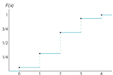
The graph of the cumulative distribution function of Example 3.9, which ap-pears as a step function in Figure 3.3, is obtained by plotting the points (x, F(x)). Certain probability distributions are applicable to more than one physical situ-ation. The probability distribution of Example 3.9, for example, also applies to the random variableY, whereY is the number of heads when a coin is tossed 4 times, or to the random variableW, whereW is the number of red cards that occur when 4 cards are drawn at random from a deck in succession with each card replaced and the deck shuffled before the next drawing. Special discrete distributions that can be applied to many different experimental situations will be considered in Chapter 5.
F(x)
x
1/4 1/2 3/4 1
0 1 2 3 4
Figure 3.3: Discrete cumulative distribution function.
3.3
Continuous Probability Distributions
At first this may seem startling, but it becomes more plausible when we consider a particular example. Let us discuss a random variable whose values are the heights of all people over 21 years of age. Between any two values, say 163.5 and 164.5 centimeters, or even 163.99 and 164.01 centimeters, there are an infinite number of heights, one of which is 164 centimeters. The probability of selecting a person at random who is exactly 164 centimeters tall and not one of the infinitely large set of heights so close to 164 centimeters that you cannot humanly measure the difference is remote, and thus we assign a probability of 0 to the event. This is not the case, however, if we talk about the probability of selecting a person who is at least 163 centimeters but not more than 165 centimeters tall. Now we are dealing with an interval rather than a point value of our random variable.
We shall concern ourselves with computing probabilities for various intervals of continuous random variables such asP(a < X < b),P(W ≥c), and so forth. Note that when X is continuous,
P(a < X ≤b) =P(a < X < b) +P(X =b) =P(a < X < b).
That is, it does not matter whether we include an endpoint of the interval or not. This is not true, though, when X is discrete.
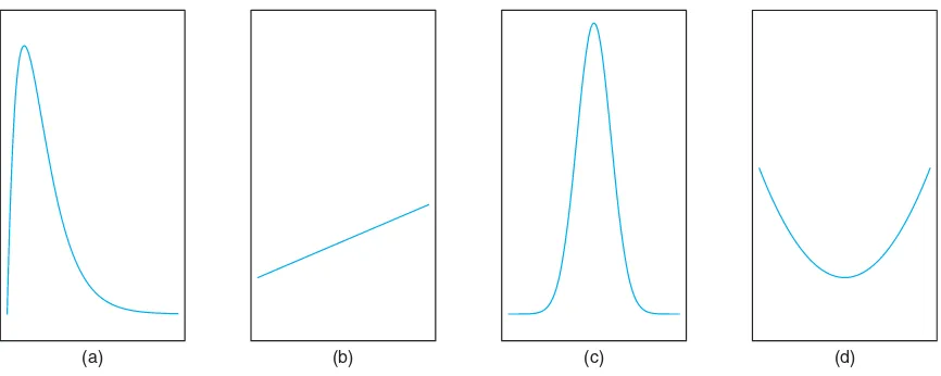
Although the probability distribution of a continuous random variable cannot be presented in tabular form, it can be stated as a formula. Such a formula would necessarily be a function of the numerical values of the continuous random variable X and as such will be represented by the functional notationf(x). In dealing with continuous variables,f(x) is usually called theprobability density function, or simply thedensity function, of X. SinceX is defined over a continuous sample space, it is possible for f(x) to have a finite number of discontinuities. However, most density functions that have practical applications in the analysis of statistical data are continuous and their graphs may take any of several forms, some of which are shown in Figure 3.4. Because areas will be used to represent probabilities and probabilities are positive numerical values, the density function must lie entirely above the xaxis.
(a) (b) (c) (d)
Figure 3.4: Typical density functions.
3.3 Continuous Probability Distributions 89
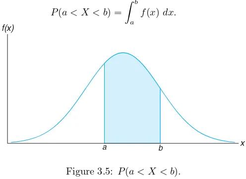
bounded by thexaxis is equal to 1 when computed over the range ofX for which f(x) is defined. Should this range ofX be a finite interval, it is always possible to extend the interval to include the entire set of real numbers by definingf(x) to be zero at all points in the extended portions of the interval. In Figure 3.5, the probability that X assumes a value betweena and b is equal to the shaded area under the density function between the ordinates at x=a and x=b, and from integral calculus is given by
P(a < X < b) =
b
a
f(x)dx.
a b x
f(x)
Figure 3.5: P(a < X < b).
Definition 3.6: The function f(x) is aprobability density function(pdf) for the continuous random variableX, defined over the set of real numbers, if
1. f(x)≥0, for allx∈R.
2. ∞
−∞f(x)dx= 1.
3. P(a < X < b) =b
a f(x)dx.
Example 3.11: Suppose that the error in the reaction temperature, in◦C, for a controlled
labora-tory experiment is a continuous random variableX having the probability density function
f(x) =
x2
3, −1< x <2, 0, elsewhere. .
(a) Verify thatf(x) is a density function. (b) FindP(0< X≤1).
Solution:We use Definition 3.6.
(a) Obviously,f(x)≥0. To verify condition 2 in Definition 3.6, we have
∞
−∞
f(x)dx=
2
−1 x2
3 dx= x3
9 | 2
−1= 8 9+
(b) Using formula 3 in Definition 3.6, we obtain
Definition 3.7: Thecumulative distribution functionF(x) of a continuous random variable X with density functionf(x) is
F(x) =P(X ≤x) =
x
−∞
f(t)dt, for − ∞< x <∞.
As an immediate consequence of Definition 3.7, one can write the two results
P(a < X < b) =F(b)−F(a) andf(x) =dF(x) dx , if the derivative exists.
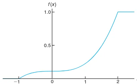
Example 3.12: For the density function of Example 3.11, find F(x), and use it to evaluate P(0< X≤1).
The cumulative distribution functionF(x) is expressed in Figure 3.6. Now
P(0< X ≤1) =F(1)−F(0) = 2
which agrees with the result obtained by using the density function in Example 3.11.
Example 3.13: The Department of Energy (DOE) puts projects out on bid and generally estimates what a reasonable bid should be. Call the estimate b. The DOE has determined that the density function of the winning (low) bid is
f(y) =
FindF(y) and use it to determine the probability that the winning bid is less than the DOE’s preliminary estimate b.
/ /
Exercises 91
f(x)
x
0 2
⫺1 1
0.5 1.0
Figure 3.6: Continuous cumulative distribution function.
Thus,
F(y) =
⎧ ⎪ ⎨
⎪ ⎩
0, y < 2 5b, 5y
8b −
1 4,
2
5b≤y <2b, 1, y≥2b.
To determine the probability that the winning bid is less than the preliminary bid estimateb, we have
P(Y ≤b) =F(b) =5 8 −
1 4 =
3 8.
Exercises
3.1 Classify the following random variables as dis-crete or continuous:
X: the number of automobile accidents per year in Virginia.
Y: the length of time to play 18 holes of golf.
M: the amount of milk produced yearly by a par-ticular cow.
N: the number of eggs laid each month by a hen.
P: the number of building permits issued each month in a certain city.
Q: the weight of grain produced per acre.
3.2 An overseas shipment of 5 foreign automobiles contains 2 that have slight paint blemishes. If an agency receives 3 of these automobiles at random, list the elements of the sample spaceS, using the lettersB and N for blemished and nonblemished, respectively;
then to each sample point assign a valuexof the ran-dom variable X representing the number of automo-biles with paint blemishes purchased by the agency.
3.3 Let W be a random variable giving the number of heads minus the number of tails in three tosses of a coin. List the elements of the sample spaceS for the three tosses of the coin and to each sample point assign a valuewofW.
3.4 A coin is flipped until 3 heads in succession oc-cur. List only those elements of the sample space that require 6 or less tosses. Is this a discrete sample space? Explain.
3.5 Determine the valuecso that each of the follow-ing functions can serve as a probability distribution of the discrete random variableX:
(a)f(x) =c(x2+ 4), forx= 0,1,2,3;
(b)f(x) =c2
x 3
3−x
92 Chapter 3 Random Variables and Probability Distributions
3.6 The shelf life, in days, for bottles of a certain prescribed medicine is a random variable having the density function
f(x) =
20,000
(x+100)3, x >0,
0, elsewhere.
Find the probability that a bottle of this medicine will have a shell life of
(a) at least 200 days;
(b) anywhere from 80 to 120 days.
3.7 The total number of hours, measured in units of 100 hours, that a family runs a vacuum cleaner over a period of one year is a continuous random variableX that has the density function
f(x) =
Find the probability that over a period of one year, a family runs their vacuum cleaner
(a) less than 120 hours; (b) between 50 and 100 hours.
3.8 Find the probability distribution of the random variable W in Exercise 3.3, assuming that the coin is biased so that a head is twice as likely to occur as a tail.
3.9 The proportion of people who respond to a certain mail-order solicitation is a continuous random variable X that has the density function
f(x) = 2(x+2)
5 , 0< x <1,
0, elsewhere.
(a) Show thatP(0< X <1) = 1.
(b) Find the probability that more than 1/4 but fewer than 1/2 of the people contacted will respond to this type of solicitation.
3.10 Find a formula for the probability distribution of the random variableXrepresenting the outcome when a single die is rolled once.
3.11 A shipment of 7 television sets contains 2 de-fective sets. A hotel makes a random purchase of 3 of the sets. If xis the number of defective sets pur-chased by the hotel, find the probability distribution of X. Express the results graphically as a probability histogram.
3.12 An investment firm offers its customers munici-pal bonds that mature after varying numbers of years. Given that the cumulative distribution function ofT, the number of years to maturity for a randomly se-lected bond, is
3.13 The probability distribution of X, the number of imperfections per 10 meters of a synthetic fabric in continuous rolls of uniform width, is given by
x 0 1 2 3 4
f(x) 0.41 0.37 0.16 0.05 0.01
Construct the cumulative distribution function ofX.
3.14 The waiting time, in hours, between successive speeders spotted by a radar unit is a continuous ran-dom variable with cumulative distribution function
F(x) =
0, x <0,
1−e−8x, x≥0.
Find the probability of waiting less than 12 minutes between successive speeders
(a) using the cumulative distribution function ofX; (b) using the probability density function ofX.
3.15 Find the cumulative distribution function of the random variableX representing the number of defec-tives in Exercise 3.11. Then usingF(x), find
(a)P(X = 1); (b)P(0< X≤2).
3.16 Construct a graph of the cumulative distribution function of Exercise 3.15.
3.17 A continuous random variable X that can as-sume values between x= 1 and x = 3 has a density function given byf(x) = 1/2.
(a) Show that the area under the curve is equal to 1. (b) FindP(2< X <2.5).
/ /
Exercises 93
3.18 A continuous random variable X that can as-sume values between x = 2 and x= 5 has a density function given byf(x) = 2(1 +x)/27. Find
(a)P(X <4); (b)P(3≤X <4).
3.19 For the density function of Exercise 3.17, find F(x). Use it to evaluateP(2< X <2.5).
3.20 For the density function of Exercise 3.18, find F(x), and use it to evaluateP(3≤X <4).
3.21 Consider the density function
f(x) =
3.22 Three cards are drawn in succession from a deck without replacement. Find the probability distribution for the number of spades.
3.23 Find the cumulative distribution function of the random variableW in Exercise 3.8. UsingF(w), find (a)P(W >0);
(b)P(−1≤W <3).
3.24 Find the probability distribution for the number of jazz CDs when 4 CDs are selected at random from a collection consisting of 5 jazz CDs, 2 classical CDs, and 3 rock CDs. Express your results by means of a formula.
3.25 From a box containing 4 dimes and 2 nickels, 3 coins are selected at random without replacement. Find the probability distribution for the totalT of the 3 coins. Express the probability distribution graphi-cally as a probability histogram.
3.26 From a box containing 4 black balls and 2 green balls, 3 balls are drawn in succession, each ball being replaced in the box before the next draw is made. Find the probability distribution for the number of green balls.
3.27 The time to failure in hours of an important piece of electronic equipment used in a manufactured DVD player has the density function
f(x) = 1
2000exp(−x/2000), x≥0,
0, x <0.
(a) FindF(x).
(b) Determine the probability that the component (and thus the DVD player) lasts more than 1000 hours before the component needs to be replaced. (c) Determine the probability that the component fails
before 2000 hours.
3.28 A cereal manufacturer is aware that the weight of the product in the box varies slightly from box to box. In fact, considerable historical data have al-lowed the determination of the density function that describes the probability structure for the weight (in ounces). LettingX be the random variable weight, in ounces, the density function can be described as
f(x) = 2
5, 23.75≤x≤26.25,
0, elsewhere.
(a) Verify that this is a valid density function. (b) Determine the probability that the weight is
smaller than 24 ounces.
(c) The company desires that the weight exceeding 26 ounces be an extremely rare occurrence. What is the probability that this rare occurrence does ac-tually occur?
3.29 An important factor in solid missile fuel is the particle size distribution. Significant problems occur if the particle sizes are too large. From production data in the past, it has been determined that the particle size (in micrometers) distribution is characterized by
f(x) =
3x−4, x >1,
0, elsewhere.
(a) Verify that this is a valid density function. (b) EvaluateF(x).
(c) What is the probability that a random particle from the manufactured fuel exceeds 4 micrometers?
3.30 Measurements of scientific systems are always subject to variation, some more than others. There are many structures for measurement error, and statis-ticians spend a great deal of time modeling these errors. Suppose the measurement errorXof a certain physical quantity is decided by the density function
f(x) =
k(3−x2), −1≤x≤1,
0, elsewhere.
(a) Determinekthat rendersf(x) a valid density func-tion.
(b) Find the probability that a random error in mea-surement is less than 1/2.
3.31 Based on extensive testing, it is determined by the manufacturer of a washing machine that the time Y (in years) before a major repair is required is char-acterized by the probability density function
f(y) =
(a) Critics would certainly consider the product a bar-gain if it is unlikely to require a major repair before the sixth year. Comment on this by determining P(Y >6).
(b) What is the probability that a major repair occurs in the first year?
3.32 The proportion of the budget for a certain type of industrial company that is allotted to environmental and pollution control is coming under scrutiny. A data collection project determines that the distribution of these proportions is given by
f(y) = 5(1
−y)4, 0≤y≤1,
0, elsewhere.
(a) Verify that the above is a valid density function. (b) What is the probability that a company chosen at
random expends less than 10% of its budget on en-vironmental and pollution controls?
(c) What is the probability that a company selected at random spends more than 50% of its budget on environmental and pollution controls?
3.33 Suppose a certain type of small data processing firm is so specialized that some have difficulty making a profit in their first year of operation. The probabil-ity densprobabil-ity function that characterizes the proportion Y that make a profit is given by
f(y) =
ky4(1−y)3, 0≤y≤1,
0, elsewhere.
(a) What is the value of k that renders the above a valid density function?
(b) Find the probability that at most 50% of the firms make a profit in the first year.
(c) Find the probability that at least 80% of the firms make a profit in the first year.
3.34 Magnetron tubes are produced on an automated assembly line. A sampling plan is used periodically to assess quality of the lengths of the tubes. This mea-surement is subject to uncertainty. It is thought that the probability that a random tube meets length spec-ification is 0.99. A sampling plan is used in which the lengths of 5 random tubes are measured.
(a) Show that the probability function ofY, the num-ber out of 5 that meet length specification, is given by the following discrete probability function:
f(y) = 5!
y!(5−y)!(0.99)
y(0.01)5−y,
fory= 0,1,2,3,4,5.
(b) Suppose random selections are made off the line and 3 are outside specifications. Usef(y) above ei-ther to support or to refute the conjecture that the probability is 0.99 that a single tube meets specifi-cations.
3.35 Suppose it is known from large amounts of his-torical data thatX, the number of cars that arrive at a specific intersection during a 20-second time period, is characterized by the following discrete probability function:
f(x) =e−66 x
x!, forx= 0,1,2, . . . .
(a) Find the probability that in a specific 20-second time period, more than 8 cars arrive at the intersection.
(b) Find the probability that only 2 cars arrive.
3.36 On a laboratory assignment, if the equipment is working, the density function of the observed outcome, X, is
(b) What is the probability thatX will exceed 0.5? (c) Given thatX ≥0.5, what is the probability that
X will be less than 0.75?
3.4
Joint Probability Distributions
simulta-3.4 Joint Probability Distributions 95
neous outcomes of several random variables. For example, we might measure the amount of precipitate P and volumeV of gas released from a controlled chemical experiment, giving rise to a two-dimensional sample space consisting of the out-comes (p, v), or we might be interested in the hardness Hand tensile strength T of cold-drawn copper, resulting in the outcomes (h, t). In a study to determine the likelihood of success in college based on high school data, we might use a three-dimensional sample space and record for each individual his or her aptitude test score, high school class rank, and grade-point average at the end of freshman year in college.
IfX and Y are two discrete random variables, the probability distribution for their simultaneous occurrence can be represented by a function with valuesf(x, y) for any pair of values (x, y) within the range of the random variablesX andY. It is customary to refer to this function as the joint probability distribution of X andY.
Hence, in the discrete case,
f(x, y) =P(X=x, Y =y);
that is, the values f(x, y) give the probability that outcomes x and y occur at the same time. For example, if an 18-wheeler is to have its tires serviced and X represents the number of miles these tires have been driven and Y represents the number of tires that need to be replaced, then f(30000,5) is the probability that the tires are used over 30,000 miles and the truck needs 5 new tires.
Definition 3.8: The functionf(x, y) is ajoint probability distributionorprobability mass
functionof the discrete random variablesX and Y if
1. f(x, y)≥0 for all (x, y),
2.
x
y
f(x, y) = 1,
3. P(X=x, Y =y) =f(x, y).
For any regionAin thexy plane,P[(X, Y)∈A] =
A
f(x, y).
Example 3.14: Two ballpoint pens are selected at random from a box that contains 3 blue pens, 2 red pens, and 3 green pens. If X is the number of blue pens selected andY is the number of red pens selected, find
(a) the joint probability functionf(x, y),
(b) P[(X, Y)∈A], whereAis the region{(x, y)|x+y≤1}.
Solution:The possible pairs of values (x, y) are (0,0), (0,1), (1,0), (1,1), (0,2), and (2,0). (a) Now,f(0,1), for example, represents the probability that a red and a green
pens are selected. The total number of equally likely ways of selecting any 2 pens from the 8 is 8
2
= 28. The number of ways of selecting 1 red from 2 red pens and 1 green from 3 green pens is2
1 3
1
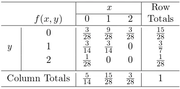
5, it will become clear that the joint probability distribution of Table 3.1 can be represented by the formula
f(x, y) =
3
x
2
y
3 2−x−y
8 2
,
forx= 0, 1, 2;y = 0, 1, 2; and 0≤x+y≤2. (b) The probability that (X, Y) fall in the regionAis
P[(X, Y)∈A] =P(X+Y ≤1) =f(0,0) +f(0,1) +f(1,0)
= 3 28+
3 14+
9 28 =
9 14.
Table 3.1: Joint Probability Distribution for Example 3.14
x Row
f(x, y) 0 1 2 Totals
0 3
28 9 28
3 28
15 28
y 1 3
14 3
14 0
3 7 2 281 0 0 281
Column Totals 5 14
15 28
3
28 1
WhenX andY are continuous random variables, thejoint density function
f(x, y) is a surface lying above the xy plane, andP[(X, Y)∈A], where Ais any region in thexyplane, is equal to the volume of the right cylinder bounded by the base Aand the surface.
Definition 3.9: The function f(x, y) is a joint density function of the continuous random variablesX andY if
1. f(x, y)≥0, for all (x, y),
2. ∞
−∞
∞
−∞f(x, y)dx dy= 1,
3. P[(X, Y)∈A] = Af(x, y)dx dy,for any regionAin the xyplane.
Example 3.15: A privately owned business operates both a drive-in facility and a walk-in facility. On a randomly selected day, let X andY, respectively, be the proportions of the time that the drive-in and the walk-in facilities are in use, and suppose that the joint density function of these random variables is
f(x, y) =
2
5(2x+ 3y), 0≤x≤1,0≤y≤1, 0, elsewhere.
(a) Verify condition 2 of Definition 3.9.
(b) FindP[(X, Y)∈A], whereA={(x, y)|0< x < 1 2,
1 4 < y <
3.4 Joint Probability Distributions 97
Solution: (a) The integration off(x, y) over the whole region is
∞
(b) To calculate the probability, we use
P[(X, Y)∈A] =P
Given the joint probability distributionf(x, y) of the discrete random variables X and Y, the probability distribution g(x) of X alone is obtained by summing f(x, y) over the values ofY. Similarly, the probability distributionh(y) ofY alone is obtained by summingf(x, y) over the values ofX. We defineg(x) andh(y) to be the marginal distributions of X and Y, respectively. When X and Y are continuous random variables, summations are replaced by integrals. We can now make the following general definition.
Definition 3.10: The marginal distributionsofX alone and ofY alone are
g(x) =
y
f(x, y) and h(y) =
x
f(x, y)
for the discrete case, and
g(x) =
for the continuous case.
Example 3.16: Show that the column and row totals of Table 3.1 give the marginal distribution of X alone and ofY alone.
Solution:For the random variableX, we see that
g(0) =f(0,0) +f(0,1) +f(0,2) = 3
which are just the column totals of Table 3.1. In a similar manner we could show that the values ofh(y) are given by the row totals. In tabular form, these marginal distributions may be written as follows:
x 0 1 2
g(x) 145 1528 283
y 0 1 2
h(y) 1528 37 281
Example 3.17: Findg(x) andh(y) for the joint density function of Example 3.15. Solution:By definition,
g(x) =
The fact that the marginal distributionsg(x) and h(y) are indeed the proba-bility distributions of the individual variables X and Y alone can be verified by showing that the conditions of Definition 3.4 or Definition 3.6 are satisfied. For example, in the continuous case
∞
In Section 3.1, we stated that the valuexof the random variableX represents an event that is a subset of the sample space. If we use the definition of conditional probability as stated in Chapter 2,
P(B|A) = P(A∩B)
3.4 Joint Probability Distributions 99
whereAandBare now the events defined byX=xandY =y, respectively, then
P(Y =y |X =x) =P(X =x, Y =y)
P(X =x) =
f(x, y)
g(x) , providedg(x)>0,
whereX andY are discrete random variables.
It is not difficult to show that the functionf(x, y)/g(x), which is strictly a func-tion ofywithxfixed, satisfies all the conditions of a probability distribution. This is also true whenf(x, y) andg(x) are the joint density and marginal distribution, respectively, of continuous random variables. As a result, it is extremely important that we make use of the special type of distribution of the form f(x, y)/g(x) in order to be able to effectively compute conditional probabilities. This type of dis-tribution is called aconditional probability distribution; the formal definition follows.
Definition 3.11: LetX andY be two random variables, discrete or continuous. Theconditional distributionof the random variableY given thatX =xis
f(y|x) = f(x, y)
g(x) , providedg(x)>0.
Similarly, the conditional distribution ofX given that Y =yis
f(x|y) = f(x, y)
h(y) , providedh(y)>0.
If we wish to find the probability that the discrete random variableX falls between aandb when it is known that the discrete variableY =y, we evaluate
P(a < X < b|Y =y) =
a<x<b
f(x|y),
where the summation extends over all values ofX betweenaandb. WhenX and Y are continuous, we evaluate
P(a < X < b|Y =y) =
b
a
f(x|y)dx.
Example 3.18: Referring to Example 3.14, find the conditional distribution ofX, given thatY = 1, and use it to determineP(X= 0 |Y = 1).
Solution:We need to findf(x|y), wherey= 1. First, we find that
h(1) = 2
x=0
f(x,1) = 3 14+
3 14+ 0 =
3 7.
Now
f(x|1) = f(x,1) h(1) =
7
3
Therefore,
and the conditional distribution ofX, given thatY = 1, is
x 0 1 2
Therefore, if it is known that 1 of the 2 pen refills selected is red, we have a probability equal to 1/2 that the other refill is not blue.
Example 3.19: The joint density for the random variables (X, Y), whereXis the unit temperature change and Y is the proportion of spectrum shift that a certain atomic particle produces, is
f(x, y) =
10xy2, 0< x < y <1, 0, elsewhere.
(a) Find the marginal densitiesg(x),h(y), and the conditional densityf(y|x). (b) Find the probability that the spectrum shifts more than half of the total
observations, given that the temperature is increased by 0.25 unit.
Solution: (a) By definition,
g(x) =
Example 3.20: Given the joint density function
f(x, y) =
x(1+3y2
)
3.4 Joint Probability Distributions 101
findg(x),h(y),f(x|y), and evaluateP(14 < X < 12 |Y = 13). Solution:By definition of the marginal density. for 0< x <2,
g(x) =
Therefore, using the conditional density definition, for 0< x <2,
f(x|y) = f(x, y) andf(x, y) =g(x)h(y). The proof follows by substituting
f(x, y) =f(x|y)h(y)
into the marginal distribution ofX. That is,
g(x) =
sinceh(y) is the probability density function ofY. Therefore,
It should make sense to the reader that iff(x|y) does not depend ony, then of course the outcome of the random variableY has no impact on the outcome of the random variableX. In other words, we say thatX andY are independent random variables. We now offer the following formal definition of statistical independence.
Definition 3.12: LetX andY be two random variables, discrete or continuous, with joint proba-bility distributionf(x, y) and marginal distributionsg(x) andh(y), respectively. The random variablesX andY are said to bestatistically independentif and only if
f(x, y) =g(x)h(y)
for all (x, y) within their range.
The continuous random variables of Example 3.20 are statistically indepen-dent, since the product of the two marginal distributions gives the joint density function. This is obviously not the case, however, for the continuous variables of Example 3.19. Checking for statistical independence of discrete random variables requires a more thorough investigation, since it is possible to have the product of the marginal distributions equal to the joint probability distribution for some but not all combinations of (x, y). If you can find any point (x, y) for whichf(x, y) is defined such that f(x, y) = g(x)h(y), the discrete variables X and Y are not statistically independent.
Example 3.21: Show that the random variables of Example 3.14 are not statistically independent. Proof: Let us consider the point (0,1). From Table 3.1 we find the three probabilities
f(0,1), g(0), and h(1) to be
f(0,1) = 3 14,
g(0) = 2
y=0
f(0, y) = 3 28+
3 14+
1 28 =
5 14,
h(1) = 2
x=0
f(x,1) = 3 14+
3 14+ 0 =
3 7.
Clearly,
f(0,1)=g(0)h(1),
and thereforeX andY are not statistically independent.
All the preceding definitions concerning two random variables can be general-ized to the case ofnrandom variables. Letf(x1, x2, . . . , xn) be the joint probability
function of the random variablesX1, X2, . . . , Xn. The marginal distribution ofX1, for example, is
g(x1) =
x2
· · ·
xn
3.4 Joint Probability Distributions 103
for the discrete case, and
g(x1) = ∞
−∞
· · ·
∞
−∞
f(x1, x2, . . . , xn)dx2 dx3· · ·dxn
for the continuous case. We can now obtain joint marginal distributionssuch as g(x1, x2), where
g(x1, x2) = ⎧ ⎨
⎩
x3
· · ·
xn
f(x1, x2, . . . , xn) (discrete case),
∞
−∞· · ·
∞
−∞f(x1, x2, . . . , xn)dx3dx4· · ·dxn (continuous case).
We could consider numerous conditional distributions. For example, thejoint con-ditional distributionofX1,X2, andX3, given thatX4=x4, X5=x5, . . . , Xn=
xn, is written
f(x1, x2, x3| x4, x5, . . . , xn) =
f(x1, x2, . . . , xn)
g(x4, x5, . . . , xn)
,
where g(x4, x5, . . . , xn) is the joint marginal distribution of the random variables
X4, X5, . . . , Xn.
A generalization of Definition 3.12 leads to the following definition for the mu-tual statistical independence of the variablesX1, X2, . . . , Xn.
Definition 3.13: Let X1, X2, . . . , Xn be n random variables, discrete or continuous, with joint probability distribution f(x1, x2, . . . , xn) and marginal distribution
f1(x1), f2(x2), . . . , fn(xn), respectively. The random variablesX1, X2, . . . , Xnare
said to be mutuallystatistically independentif and only if
f(x1, x2, . . . , xn) =f1(x1)f2(x2)· · ·fn(xn)
for all (x1, x2, . . . , xn) within their range.
Example 3.22: Suppose that the shelf life, in years, of a certain perishable food product packaged in cardboard containers is a random variable whose probability density function is given by
f(x) =
e−x, x >0,
0, elsewhere.
LetX1, X2, andX3 represent the shelf lives for three of these containers selected independently and findP(X1<2,1< X2<3, X3>2).
Solution:Since the containers were selected independently, we can assume that the random variablesX1,X2, andX3are statistically independent, having the joint probability density
f(x1, x2, x3) =f(x1)f(x2)f(x3) =e−x1e−x2e−x3 =e−x1−x2−x3, forx1>0,x2>0,x3>0, andf(x1, x2, x3) = 0 elsewhere. Hence
P(X1<2,1< X2<3, X3>2) = ∞
2 3
1 2
0
e−x1−x2−x3
dx1 dx2 dx3
104 Chapter 3 Random Variables and Probability Distributions
What Are Important Characteristics of Probability Distributions
and Where Do They Come From?
This is an important point in the text to provide the reader with a transition into the next three chapters. We have given illustrations in both examples and exercises of practical scientific and engineering situations in which probability distributions and their properties are used to solve important problems. These probability dis-tributions, either discrete or continuous, were introduced through phrases like “it is known that” or “suppose that” or even in some cases “historical evidence sug-gests that.” These are situations in which the nature of the distribution and even a good estimate of the probability structure can be determined through historical data, data from long-term studies, or even large amounts of planned data. The reader should remember the discussion of the use of histograms in Chapter 1 and from that recall how frequency distributions are estimated from the histograms. However, not all probability functions and probability density functions are derived from large amounts of historical data. There are a substantial number of situa-tions in which the nature of the scientific scenario suggests a distribution type. Indeed, many of these are reflected in exercises in both Chapter 2 and this chap-ter. When independent repeated observations are binary in nature (e.g., defective or not, survive or not, allergic or not) with value 0 or 1, the distribution covering this situation is called the binomial distribution and the probability function is known and will be demonstrated in its generality in Chapter 5. Exercise 3.34 in Section 3.3 and Review Exercise 3.80 are examples, and there are others that the reader should recognize. The scenario of a continuous distribution in time to failure, as in Review Exercise 3.69 or Exercise 3.27 on page 93, often suggests a dis-tribution type called the exponential distribution. These types of illustrations are merely two of many so-called standard distributions that are used extensively in real-world problems because the scientific scenario that gives rise to each of them is recognizable and occurs often in practice. Chapters 5 and 6 cover many of these types along with some underlying theory concerning their use.
A second part of this transition to material in future chapters deals with the notion of population parameters or distributional parameters. Recall in Chapter 1 we discussed the need to use data to provide information about these parameters. We went to some length in discussing the notions of a mean and
variance and provided a vision for the concepts in the context of a population. Indeed, the population mean and variance are easily found from the probability function for the discrete case or probability density function for the continuous case. These parameters and their importance in the solution of many types of real-world problems will provide much of the material in Chapters 8 through 17.
Exercises
3.37 Determine the values of c so that the follow-ing functions represent joint probability distributions of the random variablesX andY:
(a)f(x, y) =cxy, forx= 1,2,3;y= 1,2,3; (b)f(x, y) =c|x−y|, forx=−2,0,2;y=−2,3.
3.38 If the joint probability distribution ofX andY is given by
f(x, y) =x+y
30 , forx= 0,1,2,3; y= 0,1,2,
/ /
3.39 From a sack of fruit containing 3 oranges, 2 ap-ples, and 3 bananas, a random sample of 4 pieces of fruit is selected. IfX is the number of oranges andY is the number of apples in the sample, find
(a) the joint probability distribution of X andY; (b)P[(X, Y)∈A], whereAis the region that is given
by{(x, y)|x+y≤2}.
3.40 A fast-food restaurant operates both a drive-through facility and a walk-in facility. On a randomly selected day, letX andY, respectively, be the propor-tions of the time that the drive-through and walk-in facilities are in use, and suppose that the joint density function of these random variables is
f(x, y) = 2
3(x+ 2y), 0≤x≤1, 0≤y≤1,
0, elsewhere.
(a) Find the marginal density ofX. (b) Find the marginal density ofY.
(c) Find the probability that the drive-through facility is busy less than one-half of the time.
3.41 A candy company distributes boxes of choco-lates with a mixture of creams, toffees, and cordials. Suppose that the weight of each box is 1 kilogram, but the individual weights of the creams, toffees, and cor-dials vary from box to box. For a randomly selected box, letX andY represent the weights of the creams and the toffees, respectively, and suppose that the joint density function of these variables is
f(x, y) =
24xy, 0≤x≤1, 0≤y≤1, x+y≤1,
0, elsewhere.
(a) Find the probability that in a given box the cordials account for more than 1/2 of the weight.
(b) Find the marginal density for the weight of the creams.
(c) Find the probability that the weight of the toffees in a box is less than 1/8 of a kilogram if it is known that creams constitute 3/4 of the weight.
3.42 LetX andY denote the lengths of life, in years, of two components in an electronic system. If the joint density function of these variables is
f(x, y) =
e−(x+y), x >0, y >0,
0, elsewhere,
findP(0< X <1|Y = 2).
3.43 Let X denote the reaction time, in seconds, to a certain stimulus andY denote the temperature (◦F) at which a certain reaction starts to take place. Sup-pose that two random variablesXandY have the joint density
3.44 Each rear tire on an experimental airplane is supposed to be filled to a pressure of 40 pounds per square inch (psi). LetXdenote the actual air pressure for the right tire andY denote the actual air pressure for the left tire. Suppose thatX and Y are random variables with the joint density function
f(x, y) =
(c) Find the probability that both tires are underfilled.
3.45 LetX denote the diameter of an armored elec-tric cable andY denote the diameter of the ceramic mold that makes the cable. BothX andY are scaled so that they range between 0 and 1. Suppose thatX andY have the joint density
f(x, y) = 1
y, 0< x < y <1, 0, elsewhere.
FindP(X+Y >1/2).
3.46 Referring to Exercise 3.38, find (a) the marginal distribution ofX; (b) the marginal distribution ofY.
3.47 The amount of kerosene, in thousands of liters, in a tank at the beginning of any day is a random amountY from which a random amountX is sold dur-ing that day. Suppose that the tank is not resupplied during the day so thatx ≤ y, and assume that the joint density function of these variables is
f(x, y) =
2, 0< x≤y <1, 0, elsewhere.
106 Chapter 3 Random Variables and Probability Distributions
(b) FindP(1/4< X <1/2|Y = 3/4).
3.48 Referring to Exercise 3.39, find (a)f(y|2) for all values ofy;
(b)P(Y = 0|X= 2).
3.49 LetXdenote the number of times a certain nu-merical control machine will malfunction: 1, 2, or 3 times on any given day. LetY denote the number of times a technician is called on an emergency call. Their joint probability distribution is given as
x (a) Evaluate the marginal distribution ofX. (b) Evaluate the marginal distribution ofY. (c) FindP(Y = 3|X = 2).
3.50 Suppose thatX andY have the following joint probability distribution:
(a) Find the marginal distribution ofX. (b) Find the marginal distribution ofY.
3.51 Three cards are drawn without replacement from the 12 face cards (jacks, queens, and kings) of an ordinary deck of 52 playing cards. Let X be the number of kings selected and Y the number of jacks. Find
(a) the joint probability distribution ofX andY; (b)P[(X, Y) ∈ A], where A is the region given by
{(x, y)|x+y≥2}.
3.52 A coin is tossed twice. LetZdenote the number of heads on the first toss and W the total number of heads on the 2 tosses. If the coin is unbalanced and a head has a 40% chance of occurring, find
(a) the joint probability distribution ofW andZ; (b) the marginal distribution ofW;
(c) the marginal distribution ofZ;
(d) the probability that at least 1 head occurs.
3.53 Given the joint density function
f(x, y) =
6−x−y
8 , 0< x <2, 2< y <4,
0, elsewhere,
findP(1< Y <3|X = 1).
3.54 Determine whether the two random variables of Exercise 3.49 are dependent or independent.
3.55 Determine whether the two random variables of Exercise 3.50 are dependent or independent.
3.56 The joint density function of the random vari-ablesX andY is
f(x, y) =
6x, 0< x <1, 0< y <1
−x, 0, elsewhere.
(a) Show thatX andY are not independent. (b) FindP(X >0.3|Y = 0.5).
3.57 LetX,Y, andZhave the joint probability den-sity function
3.58 Determine whether the two random variables of Exercise 3.43 are dependent or independent.
3.59 Determine whether the two random variables of Exercise 3.44 are dependent or independent.
3.60 The joint probability density function of the ran-dom variablesX,Y, andZ is
(a) the joint marginal density function ofY andZ; (b) the marginal density ofY;
/ /
Review Exercises 107
Review Exercises
3.61 A tobacco company produces blends of tobacco, with each blend containing various proportions of Turkish, domestic, and other tobaccos. The propor-tions of Turkish and domestic in a blend are random variables with joint density function (X = Turkish and Y = domestic)
f(x, y) =
24xy, 0≤x, y≤1, x+y≤1,
0, elsewhere.
(a) Find the probability that in a given box the Turkish tobacco accounts for over half the blend.
(b) Find the marginal density function for the propor-tion of the domestic tobacco.
(c) Find the probability that the proportion of Turk-ish tobacco is less than 1/8 if it is known that the blend contains 3/4 domestic tobacco.
3.62 An insurance company offers its policyholders a number of different premium payment options. For a randomly selected policyholder, letXbe the number of months between successive payments. The cumulative distribution function ofX is
F(x) =
(a) What is the probability mass function ofX? (b) ComputeP(4< X≤7).
3.63 Two electronic components of a missile system work in harmony for the success of the total system. LetX andY denote the life in hours of the two com-ponents. The joint density ofX andY is
f(x, y) =
ye−y(1+x), x, y≥0,
0, elsewhere.
(a) Give the marginal density functions for both ran-dom variables.
(b) What is the probability that the lives of both com-ponents will exceed 2 hours?
3.64 A service facility operates with two service lines. On a randomly selected day, letXbe the proportion of time that the first line is in use whereasY is the pro-portion of time that the second line is in use. Suppose that the joint probability density function for (X, Y) is
f(x, y) =
(a) Compute the probability that neither line is busy more than half the time.
(b) Find the probability that the first line is busy more than 75% of the time.
3.65 Let the number of phone calls received by a switchboard during a 5-minute interval be a random variableX with probability function
f(x) = e −22x
x! , forx= 0,1,2, . . . .
(a) Determine the probability thatX equals 0, 1, 2, 3, 4, 5, and 6.
(b) Graph the probability mass function for these val-ues ofx.
(c) Determine the cumulative distribution function for these values ofX.
3.66 Consider the random variables X and Y with joint density function
f(x, y) =
x+y, 0≤x, y≤1,
0, elsewhere.
(a) Find the marginal distributions ofX andY. (b) FindP(X >0.5, Y >0.5).
3.67 An industrial process manufactures items that can be classified as either defective or not defective. The probability that an item is defective is 0.1. An experiment is conducted in which 5 items are drawn randomly from the process. Let the random variableX be the number of defectives in this sample of 5. What is the probability mass function ofX?
3.68 Consider the following joint probability density function of the random variablesX andY:
f(x, y) = 3x−y
9 , 1< x <3, 1< y <2,
0, elsewhere.
(a) Find the marginal density functions ofX andY. (b) AreX andY independent?
(c) FindP(X >2).
3.69 The life span in hours of an electrical compo-nent is a random variable with cumulative distribution function
F(x) =
1−e−50x, x >0,
108 Chapter 3 Random Variables and Probability Distributions
(a) Determine its probability density function. (b) Determine the probability that the life span of such
a component will exceed 70 hours.
3.70 Pairs of pants are being produced by a particu-lar outlet facility. The pants are checked by a group of 10 workers. The workers inspect pairs of pants taken randomly from the production line. Each inspector is assigned a number from 1 through 10. A buyer selects a pair of pants for purchase. Let the random variable X be the inspector number.
(a) Give a reasonable probability mass function forX. (b) Plot the cumulative distribution function forX.
3.71 The shelf life of a product is a random variable that is related to consumer acceptance. It turns out that the shelf lifeY in days of a certain type of bakery product has a density function
f(y) =
What fraction of the loaves of this product stocked to-day would you expect to be sellable 3 to-days from now?
3.72 Passenger congestion is a service problem in air-ports. Trains are installed within the airport to reduce the congestion. With the use of the train, the timeXin minutes that it takes to travel from the main terminal to a particular concourse has density function
f(x) = 1
10, 0≤x≤10,
0, elsewhere.
(a) Show that the above is a valid probability density function.
(b) Find the probability that the time it takes a pas-senger to travel from the main terminal to the con-course will not exceed 7 minutes.
3.73 Impurities in a batch of final product of a chem-ical process often reflect a serious problem. From con-siderable plant data gathered, it is known that the pro-portionY of impurities in a batch has a density func-tion given by
f(y) =
10(1−y)9, 0≤y≤1,
0, elsewhere.
(a) Verify that the above is a valid density function. (b) A batch is considered not sellable and then not
acceptable if the percentage of impurities exceeds 60%. With the current quality of the process, what is the percentage of batches that are not
acceptable?
3.74 The timeZ in minutes between calls to an elec-trical supply system has the probability density func-tion
(a) What is the probability that there are no calls within a 20-minute time interval?
(b) What is the probability that the first call comes within 10 minutes of opening?
3.75 A chemical system that results from a chemical reaction has two important components among others in a blend. The joint distribution describing the pro-portionsX1 andX2 of these two components is given
by
f(x1, x2) =
2, 0< x1< x2<1,
0, elsewhere.
(a) Give the marginal distribution ofX1.
(b) Give the marginal distribution ofX2.
(c) What is the probability that component propor-tions produce the resultsX1<0.2 andX2>0.5?
(d) Give the conditional distributionfX1|X2(x1|x2).
3.76 Consider the situation of Review Exercise 3.75. But suppose the joint distribution of the two propor-tions is given by
f(x1, x2) =
6x2, 0< x2< x1<1,
0, elsewhere.
(a) Give the marginal distributionfX1(x1) of the
pro-portionX1 and verify that it is a valid density
function.
(b) What is the probability that proportionX2 is less
than 0.5, given thatX1 is 0.7?
3.77 Consider the random variables X and Y that represent the number of vehicles that arrive at two sep-arate street corners during a certain 2-minute period. These street corners are fairly close together so it is im-portant that traffic engineers deal with them jointly if necessary. The joint distribution ofXandY is known to be
(a) Are the two random variablesX and Y indepen-dent? Explain why or why not.
3.5 Potential Misconceptions and Hazards 109
3.78 The behavior of series of components plays a huge role in scientific and engineering reliability prob-lems. The reliability of the entire system is certainly no better than that of the weakest component in the series. In a series system, the components operate in-dependently of each other. In a particular system con-taining three components, the probabilities of meeting specifications for components 1, 2, and 3, respectively, are 0.95, 0.99, and 0.92. What is the probability that the entire system works?
3.79 Another type of system that is employed in en-gineering work is a group of parallel components or a parallel system. In this more conservative approach, the probability that the system operates is larger than the probability that any component operates. The sys-tem fails only when all components fail. Consider a sit-uation in which there are 4 independent components in a parallel system with probability of operation given by
Component 1: 0.95; Component 2: 0.94; Component 3: 0.90; Component 4: 0.97.
What is the probability that the system does not fail?
3.80 Consider a system of components in which there are 5 independent components, each of which possesses an operational probability of 0.92. The system does have a redundancy built in such that it does not fail if 3 out of the 5 components are operational. What is the probability that the total system is operational?
3.81 Project: Take 5 class periods to observe the shoe color of individuals in class. Assume the shoe color categories are red, white, black, brown, and other. Complete a frequency table for each color category. (a) Estimate and interpret the meaning of the
proba-bility distribution.
(b) What is the estimated probability that in the next class period a randomly selected student will be wearing a red or a white pair of shoes?
3.5
Potential Misconceptions and Hazards;
Relationship to Material in Other Chapters
In future chapters it will become apparent that probability distributions represent the structure through which probabilities that are computed aid in the evalua-tion and understanding of a process. For example, in Review Exercise 3.65, the probability distribution that quantifies the probability of a heavy load during cer-tain time periods can be very useful in planning for any changes in the system. Review Exercise 3.69 describes a scenario in which the life span of an electronic component is studied. Knowledge of the probability structure for the component will contribute significantly to an understanding of the reliability of a large system of which the component is a part. In addition, an understanding of the general nature of probability distributions will enhance understanding of the concept of a P-value, which was introduced briefly in Chapter 1 and will play a major role beginning in Chapter 10 and extending throughout the balance of the text.