Probability & Statistics for
Engineers & Scientists
N I N T H
E D I T I O N
Ronald E. Walpole
Roanoke College
Raymond H. Myers
Virginia Tech
Sharon L. Myers
Radford University
Keying Ye
University of Texas at San Antonio
Chapter 12
Multiple Linear Regression and
Certain Nonlinear Regression
Models
12.1
Introduction
In most research problems where regression analysis is applied, more than one independent variable is needed in the regression model. The complexity of most scientific mechanisms is such that in order to be able to predict an important response, a multiple regression modelis needed. When this model is linear in the coefficients, it is called amultiple linear regression model. For the case of
kindependent variablesx1, x2, . . . , xk, the mean ofY|x1, x2, . . . , xk is given by the
multiple linear regression model
μY|x1,x2,...,xk=β0+β1x1+· · ·+βkxk,
and the estimated response is obtained from the sample regression equation
ˆ
y=b0+b1x1+· · ·+bkxk,
where each regression coefficientβi is estimated bybi from the sample data using
the method of least squares. As in the case of a single independent variable, the multiple linear regression model can often be an adequate representation of a more complicated structure within certain ranges of the independent variables.
Similar least squares techniques can also be applied for estimating the coeffi-cients when the linear model involves, say, powers and products of the independent variables. For example, whenk= 1, the experimenter may believe that the means
μY|x do not fall on a straight line but are more appropriately described by the
polynomial regression model
μY|x=β0+β1x+β2x2+· · ·+βrxr,
and the estimated response is obtained from the polynomial regression equation
ˆ
y=b0+b1x+b2x2+· · ·+brxr.
Confusion arises occasionally when we speak of a polynomial model as a linear model. However, statisticians normally refer to a linear model as one in which the parameters occur linearly, regardless of how the independent variables enter the model. An example of a nonlinear model is theexponential relationship
μY|x=αβx,
whose response is estimated by the regression equation ˆ
y=abx.
There are many phenomena in science and engineering that are inherently non-linear in nature, and when the true structure is known, an attempt should certainly be made to fit the actual model. The literature on estimation by least squares of nonlinear models is voluminous. The nonlinear models discussed in this chapter deal with nonideal conditions in which the analyst is certain that the response and hence the response model error are not normally distributed but, rather, have a binomial or Poisson distribution. These situations do occur extensively in practice. A student who wants a more general account of nonlinear regression should consult Classical and Modern Regression with Applications by Myers (1990; see the Bibliography).
12.2
Estimating the Coefficients
In this section, we obtain the least squares estimators of the parametersβ0, β1, . . . , βk
by fitting the multiple linear regression model
μY|x1,x2,...,xk =β0+β1x1+· · ·+βkxk to the data points
{(x1i, x2i, . . . , xki, yi); i= 1,2, . . . , nandn > k},
whereyiis the observed response to the valuesx1i, x2i, . . . , xkiof thekindependent
variablesx1, x2, . . . , xk. Each observation (x1i, x2i, . . . , xki, yi) is assumed to satisfy
the following equation.
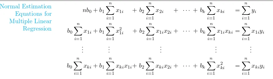
Multiple Linear Regression Model
yi=β0+β1x1i+β2x2i+· · ·+βkxki+ǫi
or
yi= ˆyi+ei=b0+b1x1i+b2x2i+· · ·+bkxki+ei,
where ǫi and ei are the random error and residual, respectively, associated with
the responseyi and fitted value ˆyi.
As in the case of simple linear regression, it is assumed that theǫiare independent
and identically distributed with mean 0 and common varianceσ2.
In using the concept of least squares to arrive at estimates b0, b1, . . . , bk, we
minimize the expression
SSE =
n
i=1 e2i =
n
i=1
(yi−b0−b1x1i−b2x2i− · · · −bkxki)2.
Differentiating SSE in turn with respect tob0, b1, . . . , bk and equating to zero, we
12.2 Estimating the Coefficients 445
solving systems of linear equations. Most statistical software can be used to obtain numerical solutions of the above equations.
Example 12.1: A study was done on a diesel-powered light-duty pickup truck to see if humidity, air temperature, and barometric pressure influence emission of nitrous oxide (in ppm). Emission measurements were taken at different times, with varying experimental conditions. The data are given in Table 12.2. The model is
μY|x1,x2,x3 =β0+β1x1+β2x2+β3x3,
or, equivalently,
yi=β0+β1x1i+β2x2i+β3x3i+ǫi, i= 1,2, . . . ,20.
Fit this multiple linear regression model to the given data and then estimate the amount of nitrous oxide emitted for the conditions where humidity is 50%, tem-perature is 76◦F, and barometric pressure is 29.30.
Table 12.1: Data for Example 12.1
Nitrous Humidity, Temp., Pressure, Nitrous Humidity, Temp., Pressure,
Oxide, y x1 x2 x3 Oxide, y x1 x2 x3 Source: Charles T. Hare, “Light-Duty Diesel Emission Correction Factors for Ambient Conditions,” EPA-600/2-77-116. U.S. Environmental Protection Agency.
Solution:The solution of the set of estimating equations yields the unique estimates
Therefore, the regression equation is
ˆ
y=−3.507778−0.002625x1+ 0.000799x2+ 0.154155x3.
For 50% humidity, a temperature of 76◦F, and a barometric pressure of 29.30, the estimated amount of nitrous oxide emitted is
ˆ
y=−3.507778−0.002625(50.0) + 0.000799(76.0) + 0.1541553(29.30) = 0.9384 ppm.
Polynomial Regression
Now suppose that we wish to fit the polynomial equation
μY|x=β0+β1x+β2x2+· · ·+βrxr
to the n pairs of observations {(xi, yi); i = 1,2, . . . , n}. Each observation, yi,
satisfies the equation
yi=β0+β1xi+β2x2i +· · ·+βrxri +ǫi
or
yi= ˆyi+ei=b0+b1xi+b2x2i +· · ·+brxri +ei,
where r is the degree of the polynomial andǫi and ei are again the random error
and residual associated with the responseyi and fitted value ˆyi, respectively. Here,
the number of pairs,n, must be at least as large asr+ 1, the number of parameters to be estimated.
Notice that the polynomial model can be considered a special case of the more general multiple linear regression model, where we setx1=x, x2=x2, . . . , xr=xr.
The normal equations assume the same form as those given on page 445. They are then solved forb0, b1, b2, . . . , br.
Example 12.2: Given the data
x 0 1 2 3 4 5 6 7 8 9
y 9.1 7.3 3.2 4.6 4.8 2.9 5.7 7.1 8.8 10.2
fit a regression curve of the formμY|x=β0+β1x+β2x2and then estimateμY|2.
Solution:From the data given, we find that
10b0+ 45b1+ 285b2= 63.7,
45b0+ 285b1+ 2025b2= 307.3,
285b0+ 2025b1+ 15,333b2= 2153.3.
Solving these normal equations, we obtain
b0= 8.698, b1=−2.341, b2= 0.288.
Therefore,
ˆ
12.3 Linear Regression Model Using Matrices 447
Whenx= 2, our estimate ofμY|2is
ˆ
y= 8.698−(2.341)(2) + (0.288)(22) = 5.168.
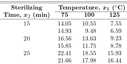
Example 12.3: The data in Table 12.2 represent the percent of impurities that resulted for various temperatures and sterilizing times during a reaction associated with the manufac-turing of a certain beverage. Estimate the regression coefficients in the polynomial model
yi=β0+β1x1i+β2x2i+β11x12i+β22x22i+β12x1ix2i+ǫi,
fori= 1,2, . . . ,18.
Table 12.2: Data for Example 12.3
Sterilizing Temperature,x1 (◦C)
Time,x2 (min) 75 100 125
15
20
25
14.05 14.93 16.56 15.85 22.41 21.66
10.55 9.48 13.63 11.75 18.55 17.98
7.55 6.59 9.23 8.78 15.93 16.44
Solution:Using the normal equations, we obtain
b0 = 56.4411, b1=−0.36190, b2=−2.75299, b11= 0.00081, b22= 0.08173, b12= 0.00314,
and our estimated regression equation is ˆ
y= 56.4411−0.36190x1−2.75299x2+ 0.00081x21+ 0.08173x22+ 0.00314x1x2.
Many of the principles and procedures associated with the estimation of poly-nomial regression functions fall into the category ofresponse surface methodol-ogy, a collection of techniques that have been used quite successfully by scientists and engineers in many fields. Thex2
i are called pure quadratic terms, and the xixj (i=j) are called interaction terms. Such problems as selecting a proper
experimental design, particularly in cases where a large number of variables are in the model, and choosing optimum operating conditions for x1, x2, . . . , xk are
often approached through the use of these methods. For an extensive exposure, the reader is referred toResponse Surface Methodology: Process and Product Opti-mization Using Designed Experimentsby Myers, Montgomery, and Anderson-Cook (2009; see the Bibliography).
12.3
Linear Regression Model Using Matrices
variables x1, x2, . . . , xk andnobservations y1, y2, . . . , yn, each of which can be
ex-pressed by the equation
yi=β0+β1x1i+β2x2i+· · ·+βkxki+ǫi.
This model essentially represents n equations describing how the response values are generated in the scientific process. Using matrix notation, we can write the following equation:
Then the least squares method for estimation ofβ, illustrated in Section 12.2, involves finding bfor which
SSE= (y−Xb)′(y−Xb)
is minimized. This minimization process involves solving for bin the equation
∂
∂b(SSE) =0.
We will not present the details regarding solution of the equations above. The result reduces to the solution of bin
(X′X)b=X′y.
Notice the nature of the X matrix. Apart from the initial element, the ith row represents the x-values that give rise to the responseyi. Writing
A=X′X=
allows the normal equations to be put in the matrix form
12.3 Linear Regression Model Using Matrices 449
If the matrix A is nonsingular, we can write the solution for the regression coefficients as
b=A−1g= (X′X)−1X′y.
Thus, we can obtain the prediction equation or regression equation by solving a set ofk+ 1 equations in a like number of unknowns. This involves the inversion of thek+ 1 byk+ 1 matrixX′X. Techniques for inverting this matrix are explained in most textbooks on elementary determinants and matrices. Of course, there are many high-speed computer packages available for multiple regression problems, packages that not only print out estimates of the regression coefficients but also provide other information relevant to making inferences concerning the regression equation.
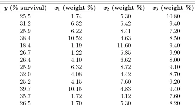
Example 12.4: The percent survival rate of sperm in a certain type of animal semen, after storage, was measured at various combinations of concentrations of three materials used to increase chance of survival. The data are given in Table 12.3. Estimate the multiple linear regression model for the given data.
Table 12.3: Data for Example 12.4
y (% survival) x1 (weight %) x2 (weight %) x3 (weight %)
From a computer readout we obtain the elements of the inverse matrix
450 Chapter 12 Multiple Linear Regression and Certain Nonlinear Regression Models
b0= 39.1574, b1= 1.0161, b2=−1.8616, b3=−0.3433.
Hence, our estimated regression equation is
ˆ
y= 39.1574 + 1.0161x1−1.8616x2−0.3433x3.
Exercises
12.1 A set of experimental runs was made to deter-mine a way of predicting cooking time y at various values of oven widthx1 and flue temperaturex2. The
coded data were recorded as follows:
y x1 x2 Estimate the multiple linear regression equation
μY|x1,x2=β0+β1x1+β2x2.
12.2 InApplied Spectroscopy, the infrared reflectance spectra properties of a viscous liquid used in the elec-tronics industry as a lubricant were studied. The de-signed experiment consisted of the effect of band fre-quency x1 and film thickness x2 on optical density y
using a Perkin-Elmer Model 621 infrared spectrometer. (Source: Pacansky, J., England, C. D., and Wattman, R., 1986.)
Estimate the multiple linear regression equation ˆ
y=b0+b1x1+b2x2.
12.3 Suppose in Review Exercise 11.53 on page 437 that we were also given the number of class periods missed by the 12 students taking the chemistry course. The complete data are shown.
Chemistry Test Classes Student Grade,y Score,x1Missed,x2
1
(a) Fit a multiple linear regression equation of the form ˆ
y=b0+b1x1+b2x2.
(b) Estimate the chemistry grade for a student who has an intelligence test score of 60 and missed 4 classes.
12.4 An experiment was conducted to determine if the weight of an animal can be predicted after a given period of time on the basis of the initial weight of the animal and the amount of feed that was eaten. The following data, measured in kilograms, were recorded:
Final Initial Feed Weight,y Weight,x1 Weight,x2 (a) Fit a multiple regression equation of the form
μY|x1,x2 =β0+β1x1+β2x2.
(b) Predict the final weight of an animal having an ini-tial weight of 35 kilograms that is given 250 kilo-grams of feed.
12.5 The electric power consumed each month by a chemical plant is thought to be related to the average ambient temperature x1, the number of days in the
monthx2, the average product purityx3, and the tons
of product producedx4. The past year’s historical data
/ /
(a) Fit a multiple linear regression model using the above data set.
(b) Predict power consumption for a month in which
x1 = 75◦F,x2 = 24 days,x3 = 90%, andx4= 98
tons.
12.6 An experiment was conducted on a new model of a particular make of automobile to determine the stopping distance at various speeds. The following data were recorded.
Speed,v (km/hr) 35 50 65 80 95 110
Stopping Distance,d(m) 16 26 41 62 88 119 (a) Fit a multiple regression curve of the formμD|v=
β0+β1v+β2v2.
(b) Estimate the stopping distance when the car is traveling at 70 kilometers per hour.
12.7 An experiment was conducted in order to de-termine if cerebral blood flow in human beings can be predicted from arterial oxygen tension (millimeters of mercury). Fifteen patients participated in the study, and the following data were collected:
Blood Flow, Arterial Oxygen
y Tension,x
84.33 603.40 Estimate the quadratic regression equation
μY|x=β0+β1x+β2x2.
12.8 The following is a set of coded experimental data on the compressive strength of a particular alloy at var-ious values of the concentration of some additive:
Concentration, Compressive
x Strength, y
10.0 (a) Estimate the quadratic regression equationμY|x=
β0+β1x+β2x2.
(b) Test for lack of fit of the model.
12.9 (a) Fit a multiple regression equation of the formμY|x =β0+β1x1+β2x2 to the data of
Ex-ample 11.8 on page 420.
(b) Estimate the yield of the chemical reaction for a temperature of 225◦C.
12.10 The following data are given:
x 0 1 2 3 4 5 6
y 1 4 5 3 2 3 4
(a) Fit the cubic modelμY|x=β0+β1x+β2x2+β3x3.
(b) PredictY whenx= 2.
12.11 An experiment was conducted to study the size of squid eaten by sharks and tuna. The regressor vari-ables are characteristics of the beaks of the squid. The data are given as follows:
452 Chapter 12 Multiple Linear Regression and Certain Nonlinear Regression Models
In the study, the regressor variables and response con-sidered are
x1= rostral length, in inches,
x2= wing length, in inches,
x3= rostral to notch length, in inches,
x4= notch to wing length, in inches,
x5= width, in inches,
y= weight, in pounds.
Estimate the multiple linear regression equation
μY|x1,x2,x3,x4,x5
=β0+β1x1+β2x2+β3x3+β4x4+β5x5.
12.12 The following data reflect information from 17 U.S. Naval hospitals at various sites around the world. The regressors are workload variables, that is, items that result in the need for personnel in a hospital. A brief description of the variables is as follows:
y= monthly labor-hours,
x1= average daily patient load,
x2= monthly X-ray exposures,
x3= monthly occupied bed-days,
x4= eligible population in the area/1000,
x5= average length of patient’s stay, in days.
Site x1 x2 x3 x4 x5 y The goal here is to produce an empirical equation that will estimate (or predict) personnel needs for Naval hospitals. Estimate the multiple linear regression equa-tion
μY|x1,x2,x3,x4,x5
=β0+β1x1+β2x2+β3x3+β4x4+β5x5.
12.13 A study was performed on a type of bear-ing to find the relationship of amount of wear y to
x1 = oil viscosity andx2 = load. The following data
were obtained. (FromResponse Surface Methodology, Myers, Montgomery, and Anderson-Cook, 2009.)
y x1 x2 y x1 x2 (a) Estimate the unknown parameters of the multiple
linear regression equation
μY|x1,x2 =β0+β1x1+β2x2.
(b) Predict wear when oil viscosity is 20 and load is 1200.
12.14 Eleven student teachers took part in an eval-uation program designed to measure teacher effective-ness and determine what factors are important. The response measure was a quantitative evaluation of the teacher. The regressor variables were scores on four standardized tests given to each teacher. The data are as follows: Estimate the multiple linear regression equation
μY|x1,x2,x3,x4=β0+β1x1+β2x2+β3x3+β4x4.
12.15 The personnel department of a certain indus-trial firm used 12 subjects in a study to determine the relationship between job performance rating (y) and scores on four tests. The data are as follows:
y x1 x2 x3 x4
12.4 Properties of the Least Squares Estimators 453
Estimate the regression coefficients in the model ˆ
y=b0+b1x1+b2x2+b3x3+b4x4.
12.16 An engineer at a semiconductor company wants to model the relationship between the gain or hFE of a device (y) and three parameters: emitter-RS (x1), base-RS (x2), and emitter-to-base-RS (x3). The
data are shown below:
x1, x2, x3, y, Emitter-RS Base-RS E-B-RS hFE
14.62 Emitter-RS Base-RS E-B-RS hFE
16.12 (Data from Myers, Montgomery, and Anderson-Cook, 2009.)
(a) Fit a multiple linear regression to the data. (b) Predict hFE whenx1= 14,x2= 220, andx3= 5.
12.4
Properties of the Least Squares Estimators
The means and variances of the estimatorsb0, b1, . . . , bk are readily obtained under
certain assumptions on the random errorsǫ1, ǫ2, . . . , ǫk that are identical to those
made in the case of simple linear regression. When we assume these errors to be independent, each with mean 0 and varianceσ2, it can be shown thatb
0, b1, . . . , bk
are, respectively, unbiased estimators of the regression coefficients β0, β1, . . . , βk.
In addition, the variances of theb’s are obtained through the elements of the inverse of theAmatrix. Note that the off-diagonal elements of A=X′Xrepresent sums of products of elements in the columns of X, while the diagonal elements of A represent sums of squares of elements in the columns of X. The inverse matrix, A−1, apart from the multiplier σ2, represents the variance-covariance matrix
of the estimated regression coefficients. That is, the elements of the matrixA−1σ2
display the variances ofb0, b1, . . . , bk on the main diagonal and covariances on the
off-diagonal. For example, in ak= 2 multiple linear regression problem, we might write
with the elements below the main diagonal determined through the symmetry of the matrix. Then we can write
σb2i=ciiσ
Of course, the estimates of the variances and hence the standard errors of these estimators are obtained by replacing σ2 with the appropriate estimate obtained
terms of the error sum of squares, which is computed using the formula estab-lished in Theorem 12.1. In the theorem, we are making the assumptions on theǫi
described above.
Theorem 12.1: For the linear regression equation
y=Xβ+ǫ,
an unbiased estimate ofσ2 is given by the error or residual mean square
s2= SSE
n−k−1, where SSE=
n
i=1 e2i =
n
i=1
(yi−yˆi)2.
We can see that Theorem 12.1 represents a generalization of Theorem 11.1 for the simple linear regression case. The proof is left for the reader. As in the simpler linear regression case, the estimate s2 is a measure of the variation in the prediction errors or residuals. Other important inferences regarding the fitted regression equation, based on the values of the individual residuals ei = yi−yˆi, i= 1,2, . . . , n, are discussed in Sections 12.10 and 12.11.
The error and regression sums of squares take on the same form and play the same role as in the simple linear regression case. In fact, the sum-of-squares identity
n
i=1
(yi−y¯)2= n
i=1
(ˆyi−y¯)2+ n
i=1
(yi−yˆi)2
continues to hold, and we retain our previous notation, namely
SST =SSR+SSE,
with
SST =
n
i=1
(yi−y¯)2= total sum of squares
and
SSR=
n
i=1
(ˆyi−y¯)2= regression sum of squares.
There arekdegrees of freedom associated withSSR, and, as always, SST has
n−1 degrees of freedom. Therefore, after subtraction,SSE hasn−k−1 degrees of freedom. Thus, our estimate of σ2 is again given by the error sum of squares
divided by its degrees of freedom. All three of these sums of squares will appear on the printouts of most multiple regression computer packages. Note that the condition n > k in Section 12.2 guarantees that the degrees of freedom of SSE
12.5 Inferences in Multiple Linear Regression 455
Analysis of Variance in Multiple Regression
The partition of the total sum of squares into its components, the regression and error sums of squares, plays an important role. An analysis of variance can be conducted to shed light on the quality of the regression equation. A useful hypothesis that determines if a significant amount of variation is explained by the model is
H0: β1=β2=β3=· · ·=βk= 0.
The analysis of variance involves an F-test via a table given as follows:
Source Sum of Squares Degrees of Freedom Mean Squares F
Regression SSR k M SR= SSR
k f =
M SR M SE
Error SSE n−(k+ 1) M SE= n−SSE(k+1)
Total SST n−1
This test is an upper-tailed test. Rejection of H0 implies that the regression equation differs from a constant. That is, at least one regressor variable is important. More discussion of the use of analysis of variance appears in subsequent sections.
Further utility of the mean square error (or residual mean square) lies in its use in hypothesis testing and confidence interval estimation, which is discussed in Sec-tion 12.5. In addiSec-tion, the mean square error plays an important role in situaSec-tions where the scientist is searching for the best from a set of competing models. Many model-building criteria involve the statistic s2. Criteria for comparing competing
models are discussed in Section 12.11.
12.5
Inferences in Multiple Linear Regression
A knowledge of the distributions of the individual coefficient estimators enables the experimenter to construct confidence intervals for the coefficients and to test hypotheses about them. Recall from Section 12.4 that the bj (j = 0,1,2, . . . , k)
are normally distributed with meanβj and variancecjjσ2. Thus, we can use the
statistic
t=bj−βj0
s√cjj
with n−k−1 degrees of freedom to test hypotheses and construct confidence intervals onβj. For example, if we wish to test
H0: βj =βj0, H1: βj =βj0,
Example 12.5: For the model of Example 12.4, test the hypothesis that β2 = −2.5 at the 0.05
level of significance against the alternative that β2>−2.5.
Solution: H0: β2=−2.5,
H1: β2>−2.5.
Computations:
t=b2−β20
s√c22
=−1.8616 + 2.5
2.073√0.0166 = 2.390,
P =P(T >2.390) = 0.04.
Decision: RejectH0and conclude thatβ2>−2.5.
Individual
t
-Tests for Variable Screening
The t-test most often used in multiple regression is the one that tests the impor-tance of individual coefficients (i.e.,H0:βj= 0 against the alternativeH1:βj = 0).
These tests often contribute to what is termedvariable screening, where the ana-lyst attempts to arrive at the most useful model (i.e., the choice of which regressors to use). It should be emphasized here that if a coefficient is found insignificant (i.e., the hypothesisH0:βj = 0is not rejected), the conclusion drawn is that the
vari-ableis insignificant (i.e., explains an insignificant amount of variation iny),in the presence of the other regressors in the model. This point will be reaffirmed in a future discussion.
Inferences on Mean Response and Prediction
One of the most useful inferences that can be made regarding the quality of the predicted responsey0corresponding to the valuesx10, x20, . . . , xk0is the confidence
interval on the mean responseμY|x10,x20,...,xk0. We are interested in constructing a confidence interval on the mean response for the set of conditions given by
x′0= [1, x10, x20, . . . , xk0].
We augment the conditions on the x’s by the number 1 in order to facilitate the matrix notation. Normality in the ǫi produces normality in thebj and the mean
and variance are still the same as indicated in Section 12.4. So is the covariance betweenbi andbj, fori=j. Hence,
ˆ
y=b0+
k
j=1 bjxj0
is likewise normally distributed and is, in fact, an unbiased estimator for themean responseon which we are attempting to attach a confidence interval. The variance of ˆy0, written in matrix notation simply as a function of σ2, (X′X)−1, and the
condition vector x′
0, is
σy2ˆ0 =σ
2x′
12.5 Inferences in Multiple Linear Regression 457
If this expression is expanded for a given case, sayk= 2, it is readily seen that it appropriately accounts for the variance of thebj and the covariance ofbi and bj,
for i=j. After σ2 is replaced bys2 as given by Theorem 12.1, the 100(1−α)%
confidence interval onμY|x10,x20,...,xk0 can be constructed from the statistic
T = yˆ0−μY|x10,x20,...,xk0
sx′
0(X′X)−1x0 ,
which has at-distribution withn−k−1 degrees of freedom.
Confidence Interval forμY|x10,x20,...,xk0
A 100(1−α)% confidence interval for the mean responseμY|x10,x20,...,xk0 is
ˆ
y0−tα/2s 5
x′
0(X′X)−1x0< μY|x10,x20,...,xk0<yˆ0+tα/2s
5
x′
0(X′X)−1x0,
wheretα/2 is a value of thet-distribution withn−k−1 degrees of freedom.
The quantitysx′
0(X′X)−1x0 is often called thestandard error of predic-tionand appears on the printout of many regression computer packages.
Example 12.6: Using the data of Example 12.4, construct a 95% confidence interval for the mean response when x1= 3%,x2= 8%, andx3= 9%.
Solution:From the regression equation of Example 12.4, the estimated percent survival when
x1= 3%,x2= 8%, andx3= 9% is
ˆ
y= 39.1574 + (1.0161)(3)−(1.8616)(8)−(0.3433)(9) = 24.2232.
Next, we find that
x′0(X′X)−1x0= [1,3,8,9] ⎡ ⎢ ⎢ ⎣
8.0648 −0.0826 −0.0942 −0.7905
−0.0826 0.0085 0.0017 0.0037
−0.0942 0.0017 0.0166 −0.0021
−0.7905 0.0037 −0.0021 0.0886
⎤ ⎥ ⎥ ⎦ ⎡ ⎢ ⎢ ⎣
1 3 8 9
⎤ ⎥ ⎥ ⎦
= 0.1267.
Using the mean square error,s2= 4.298 ors= 2.073, and Table A.4, we see that t0.025 = 2.262 for 9 degrees of freedom. Therefore, a 95% confidence interval for
the mean percent survival for x1= 3%,x2= 8%, andx3= 9% is given by
24.2232−(2.262)(2.073)√0.1267< μY|3,8,9
<24.2232 + (2.262)(2.073)√0.1267,
or simply 22.5541< μY|3,8,9<25.8923.
As in the case of simple linear regression, we need to make a clear distinction between the confidence interval on a mean response and the prediction interval on anobserved response. The latter provides a bound within which we can say with a preselected degree of certainty that a new observed response will fall.
A prediction interval for a single predicted responsey0is once again established
by considering the difference ˆy0−y0. The sampling distribution can be shown to
be normal with mean
and variance
σ2ˆy0−y0 =σ
2[1 +x′
0(X′X)−1x0].
Thus, a 100(1−α)% prediction interval for a single prediction value y0 can be
constructed from the statistic
T = yˆ0−y0
s1 +x′
0(X′X)−1x0 ,
which has at-distribution withn−k−1 degrees of freedom. Prediction Interval
fory0
A 100(1−α)% prediction interval for asingle responsey0is given by
ˆ
y0−tα/2s 5
1 +x′
0(X′X)−1x0< y0<yˆ0+tα/2s 5
1 +x′
0(X′X)−1x0,
wheretα/2 is a value of thet-distribution withn−k−1 degrees of freedom.
Example 12.7: Using the data of Example 12.4, construct a 95% prediction interval for an indi-vidual percent survival response whenx1= 3%,x2= 8%, andx3= 9%.
Solution:Referring to the results of Example 12.6, we find that the 95% prediction interval for the responsey0, whenx1= 3%,x2= 8%, andx3= 9%, is
24.2232−(2.262)(2.073)√1.1267< y0<24.2232 + (2.262)(2.073)
√
1.1267,
which reduces to 19.2459< y0<29.2005. Notice, as expected, that the prediction
interval is considerably wider than the confidence interval for mean percent survival found in Example 12.6.
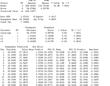
Annotated Printout for Data of Example 12.4
Figure 12.1 shows an annotated computer printout for a multiple linear regression fit to the data of Example 12.4. The package used is SAS.
Note the model parameter estimates, the standard errors, and the t-statistics shown in the output. The standard errors are computed from square roots of di-agonal elements of (X′X)−1s2. In this illustration, the variablex
3 is insignificant
in the presence of x1 andx2 based on thet-test and the correspondingP-value of
0.5916. The terms CLM and CLI are confidence intervals on mean response and prediction limits on an individual observation, respectively. Thef-test in the anal-ysis of variance indicates that a significant amount of variability is explained. As an example of the interpretation of CLM and CLI, consider observation 10. With an observation of 25.2000 and a predicted value of 26.0676, we are 95% confident that the mean response is between 24.5024 and 27.6329, and a new observation will fall between 21.1238 and 31.0114 with probability 0.95. The R2 value of 0.9117
12.5 Inferences in Multiple Linear Regression 459
Sum of Mean
Source DF Squares Square F Value Pr > F Model 3 399.45437 133.15146 30.98 <.0001 Error 9 38.67640 4.29738
Corrected Total 12 438.13077
Root MSE 2.07301 R-Square 0.9117 Dependent Mean 29.03846 Adj R-Sq 0.8823 Coeff Var 7.13885
Parameter Standard
Variable DF Estimate Error t Value Pr > |t| Intercept 1 39.15735 5.88706 6.65 <.0001 x1 1 1.01610 0.19090 5.32 0.0005 x2 1 -1.86165 0.26733 -6.96 <.0001 x3 1 -0.34326 0.61705 -0.56 0.5916
Dependent Predicted Std Error
Obs Variable Value Mean Predict 95% CL Mean 95% CL Predict Residual 1 25.5000 27.3514 1.4152 24.1500 30.5528 21.6734 33.0294 -1.8514 2 31.2000 32.2623 0.7846 30.4875 34.0371 27.2482 37.2764 -1.0623 3 25.9000 27.3495 1.3588 24.2757 30.4234 21.7425 32.9566 -1.4495 4 38.4000 38.3096 1.2818 35.4099 41.2093 32.7960 43.8232 0.0904 5 18.4000 15.5447 1.5789 11.9730 19.1165 9.6499 21.4395 2.8553 6 26.7000 26.1081 1.0358 23.7649 28.4512 20.8658 31.3503 0.5919 7 26.4000 28.2532 0.8094 26.4222 30.0841 23.2189 33.2874 -1.8532 8 25.9000 26.2219 0.9732 24.0204 28.4233 21.0414 31.4023 -0.3219 9 32.0000 32.0882 0.7828 30.3175 33.8589 27.0755 37.1008 -0.0882 10 25.2000 26.0676 0.6919 24.5024 27.6329 21.1238 31.0114 -0.8676 11 39.7000 37.2524 1.3070 34.2957 40.2090 31.7086 42.7961 2.4476 12 35.7000 32.4879 1.4648 29.1743 35.8015 26.7459 38.2300 3.2121 13 26.5000 28.2032 0.9841 25.9771 30.4294 23.0122 33.3943 -1.7032
Figure 12.1: SASprintout for data in Example 12.4.
More on Analysis of Variance in Multiple Regression (Optional)
In Section 12.4, we discussed briefly the partition of the total sum of squares
n i=1
(yi−y¯)2into its two components, the regression model and error sums of squares
(illustrated in Figure 12.1). The analysis of variance leads to a test of
H0: β1=β2=β3=· · ·=βk= 0.
Rejection of the null hypothesis has an important interpretation for the scientist or engineer. (For those who are interested in more extensive treatment of the subject using matrices, it is useful to discuss the development of these sums of squares used in ANOVA.)
First, recall in Section 12.3,b, the vector of least squares estimators, is given by
A partition of the uncorrected sum of squares
y′y=
n
i=1 yi2
into two components is given by
y′y=b′X′y+ (y′y−b′X′y)
=y′X(X′X)−1X′y+ [y′y−y′X(X′X)−1X′y].
The second term (in brackets) on the right-hand side is simply the error sum of
squares n
i=1
(yi−yˆi)2. The reader should see that an alternative expression for the
error sum of squares is
SSE=y′[In−X(X′X)−1X′]y.
The term y′X(X′X)−1
X′yis called the regression sum of squares. However,
it is not the expression
n i=1
(ˆyi−y¯)2 used for testing the “importance” of the terms b1, b2, . . . , bk but, rather,
y′X(X′X)−1X′y=
n
i=1
ˆ
yi2,
which is a regression sum of squares uncorrected for the mean. As such, it would only be used in testing if the regression equation differs significantly from zero, that is,
H0: β0=β1=β2=· · ·=βk= 0.
In general, this is not as important as testing
H0: β1=β2=· · ·=βk = 0,
since the latter states that the mean response is a constant, not necessarily zero.
Degrees of Freedom
Thus, the partition of sums of squares and degrees of freedom reduces to
Source Sum of Squares d.f.
Regression
n i=1
ˆ
y2
i =y′X(X′X)−1X′y k+ 1
Error n
i=1
(yi−yˆi)2=y′[In−X(X′X)−1X′]y n−(k+ 1)
Total
n i=1
y2
/ /
Exercises 461
Hypothesis of Interest
Now, of course, the hypotheses of interest for an ANOVA must eliminate the role of the intercept described previously. Strictly speaking, if H0: β1 = β2 =· · · = βk = 0, then the estimated regression line is merely ˆyi = ¯y. As a result, we are
actually seeking evidence that the regression equation “varies from a constant.” Thus, the total and regression sums of squares must be corrected for the mean. As a result, we have
n
i=1
(yi−y¯)2= n
i=1
(ˆyi−y¯)2+ n
i=1
(yi−yˆi)2.
In matrix notation this is simply
y′[In−1(1′1)−11′]y=y′[X(X′X)−1X′−1(1′1)−11′]y+y′[In−X(X′X)−1X′]y.
In this expression,1is a vector ofn ones. As a result, we are merely subtracting
y′1(1′1)−11′y= 1
n
n
i=1 yi
2
fromy′yand fromy′X(X′X)−1X′y(i.e., correcting the total and regression sums of squares for the mean).
Finally, the appropriate partitioning of sums of squares with degrees of freedom is as follows:
Source Sum of Squares d.f.
Regression
n i=1
(ˆyi−y¯)2=y′[X(X′X)−1X′−1(1′1)−11]y k
Error
n i=1
(yi−yˆi)2=y′[In−X(X′X)−1X′]y n−(k+ 1)
Total
n i=1
(yi−y¯)2=y′[In−1(1′1)−11′]y n−1
This is the ANOVA table that appears in the computer printout of Figure 12.1. The expression y′[1(1′1)−11′]y is often called the regression sum of squares associated with the mean, and 1 degree of freedom is allocated to it.
Exercises
12.17 For the data of Exercise 12.2 on page 450, es-timateσ2.
12.18 For the data of Exercise 12.1 on page 450, es-timateσ2.
12.19 For the data of Exercise 12.5 on page 450, es-timateσ2.
12.20 Obtain estimates of the variances and the
co-variance of the estimatorsb1andb2of Exercise 12.2 on
page 450.
12.21 Referring to Exercise 12.5 on page 450, find the estimate of
(a)σ2
b2;
(b) Cov(b1, b4).
test the hypothesis that β2 = 0 at the 0.05 level of
significance against the alternative thatβ2= 0.
12.23 For the model of Exercise 12.2 on page 450, test the hypothesis that β1 = 0 at the 0.05 level of
significance against the alternative thatβ1= 0.
12.24 For the model of Exercise 12.1 on page 450, test the hypotheses thatβ1= 2 against the alternative
thatβ1= 2. Use aP-value in your conclusion.
12.25 Using the data of Exercise 12.2 on page 450 and the estimate of σ2 from Exercise 12.17, compute 95% confidence intervals for the predicted response and the mean response whenx1= 900 andx2= 1.00.
12.26 For Exercise 12.8 on page 451, construct a 90% confidence interval for the mean compressive strength when the concentration is x = 19.5 and a quadratic model is used.
12.27 Using the data of Exercise 12.5 on page 450 and the estimate of σ2 from Exercise 12.19, compute 95% confidence intervals for the predicted response and the mean response when x1 = 75, x2 = 24, x3 = 90,
andx4= 98.
12.28 Consider the following data from Exercise 12.13 on page 452.
y(wear) x1 (oil viscosity) x2 (load)
193 1.6 851
230 15.5 816 172 22.0 1058 91 43.0 1201 113 33.0 1357 125 40.0 1115 (a) Estimate σ2 using multiple regression of y on x
1
andx2.
(b) Compute predicted values, a 95% confidence inter-val for mean wear, and a 95% prediction interinter-val for observed wear ifx1 = 20 andx2= 1000.
12.29 Using the data from Exercise 12.28, test the following at the 0.05 level.
(a)H0: β1= 0 versusH1: β1= 0;
(b)H0: β2= 0 versusH1: β2= 0.
(c) Do you have any reason to believe that the model in Exercise 12.28 should be changed? Why or why not?
12.30 Use the data from Exercise 12.16 on page 453. (a) Estimate σ2 using the multiple regression ofyon
x1,x2, andx3,
(b) Compute a 95% prediction interval for the ob-served gain with the three regressors atx1= 15.0,
x2= 220.0, andx3= 6.0.
12.6
Choice of a Fitted Model through Hypothesis Testing
In many regression situations, individual coefficients are of importance to the ex-perimenter. For example, in an economics application,β1, β2, . . . might have some
particular significance, and thus confidence intervals and tests of hypotheses on these parameters would be of interest to the economist. However, consider an in-dustrial chemical situation in which the postulated model assumes that reaction yield is linearly dependent on reaction temperature and concentration of a certain catalyst. It is probably known that this is not the true model but an adequate ap-proximation, so interest is likely to be not in the individual parameters but rather in the ability of the entire function to predict the true response in the range of the variables considered. Therefore, in this situation, one would put more emphasis on
σ2 ˆ
Y, confidence intervals on the mean response, and so forth, and likely deemphasize
inferences on individual parameters.
The experimenter using regression analysis is also interested in deletion of vari-ables when the situation dictates that, in addition to arriving at a workable pre-diction equation, he or she must find the “best regression” involving only variables that are useful predictors. There are a number of computer programs that sequen-tially arrive at the so-called best regression equation depending on certain criteria. We discuss this further in Section 12.9.
12.6 Choice of a Fitted Model through Hypothesis Testing 463
Coefficient of Determination, or
R2 R2= SSR
SST =
n i=1
(ˆyi−y¯)2
n i=1
(yi−y¯)2
= 1−SSESST.
Note that this parallels the description of R2 in Chapter 11. At this point
the explanation might be clearer since we now focus on SSR as the variability explained. The quantityR2 merely indicates what proportion of the total
vari-ation in the response Y is explained by the fitted model. Often an experimenter will report R2×100% and interpret the result as percent variation explained by
the postulated model. The square root of R2 is called themultiple correlation coefficient between Y and the set x1, x2, . . . , xk. The value of R2 for the case
in Example 12.4, indicating the proportion of variation explained by the three independent variablesx1,x2, andx3, is
R2= SSR
SST =
399.45
438.13 = 0.9117,
which means that 91.17% of the variation in percent survival has been explained by the linear regression model.
The regression sum of squares can be used to give some indication concerning whether or not the model is an adequate explanation of the true situation. We can test the hypothesisH0that theregression is not significantby merely forming
the ratio
f = SSR/k
SSE/(n−k−1) =
SSR/k s2
and rejecting H0 at theα-level of significance whenf > fα(k, n−k−1). For the
data of Example 12.4, we obtain
f = 399.45/3
4.298 = 30.98.
From the printout in Figure 12.1, theP-value is less than 0.0001. This should not be misinterpreted. Although it does indicate that the regression explained by the model is significant, this does not rule out the following possibilities:
1. The linear regression model for this set of x’s is not the only model that can be used to explain the data; indeed, there may be other models with transformations on thex’s that give a larger value of the F-statistic.
2. The model might have been more effective with the inclusion of other variables in addition to x1, x2, andx3 or perhaps with the deletion of one or more of
the variables in the model, sayx3, which has aP= 0.5916.
The reader should recall the discussion in Section 11.5 regarding the pitfalls in the use of R2 as a criterion for comparing competing models. These pitfalls
to overfit is so great. One should always keep in mind that R2 ≈1.0 can always
be achieved at the expense of error degrees of freedom when an excess of model terms is employed. However, R2 = 1, describing a model with a near perfect fit,
does not always result in a model that predicts well.
The Adjusted Coefficient of Determination (
R
2adj
)
In Chapter 11, several figures displaying computer printout from both SAS and
MINITAB featured a statistic called adjusted R2 or adjusted coefficient of
deter-mination. Adjusted R2 is a variation on R2 that provides an adjustment for degrees of freedom. The coefficient of determination as defined on page 407 cannot decrease as terms are added to the model. In other words, R2 does not
decrease as the error degrees of freedom n−k−1 are reduced, the latter result being produced by an increase in k, the number of model terms. Adjusted R2
is computed by dividingSSE andSST by their respective degrees of freedom as follows.
AdjustedR2
R2adj= 1−
SSE/(n−k−1)
SST /(n−1) .
To illustrate the use ofR2
adj, Example 12.4 will be revisited.
How Are
R
2and
R
2adj
Affected by Removal of
x
3?
Thet-test (or correspondingF-test) forx3suggests that a simpler model involving
onlyx1and x2 may well be an improvement. In other words, the complete model
with all the regressors may be an overfitted model. It is certainly of interest to investigate R2 and R2
adj for both the full (x1, x2, x3) and the reduced (x1, x2)
models. We already know that R2
full = 0.9117 from Figure 12.1. The SSE for
the reduced model is 40.01, and thus R2reduced = 1−43840..0113 = 0.9087. Thus, more
variability is explained with x3 in the model. However, as we have indicated, this
will occur even if the model is an overfitted model. Now, of course,R2
adjis designed
to provide a statistic that punishes an overfitted model, so we might expect it to favor the reduced model. Indeed, for the full model
R2adj= 1−
38.6764/9
438.1308/12 = 1− 4.2974
36.5109 = 0.8823,
whereas for the reduced model (deletion ofx3)
R2adj= 1−
40.01/10
438.1308/12 = 1− 4.001
36.5109 = 0.8904.
Thus, R2
adj does indeed favor the reduced model and confirms the evidence
12.6 Choice of a Fitted Model through Hypothesis Testing 465
Test on an Individual Coefficient
The addition of any single variable to a regression system will increase the re-gression sum of squares and thusreduce the error sum of squares. Consequently, we must decide whether the increase in regression is sufficient to warrant using the variable in the model. As we might expect, the use of unimportant variables can reduce the effectiveness of the prediction equation by increasing the variance of the estimated response. We shall pursue this point further by considering the importance ofx3 in Example 12.4. Initially, we can test
H0: β3= 0, H1: β3= 0
by using thet-distribution with 9 degrees of freedom. We have
t=b3−0
s√c33
= −0.3433
2.073√0.0886 =−0.556,
which indicates that β3 does not differ significantly from zero, and hence we may
very well feel justified in removing x3 from the model. Suppose that we consider
the regression of Y on the set (x1, x2), the least squares normal equations now
reducing to
⎡
⎣ 1359..043 39459..7255 36043 81..826621 81.82 360.6621 576.7264
⎤ ⎦ ⎡ ⎣bb01
b2 ⎤
⎦=
⎡
⎣ 1877377..505670 2246.6610
⎤ ⎦.
The estimated regression coefficients for this reduced model are
b0= 36.094, b1= 1.031, b2=−1.870,
and the resulting regression sum of squares with 2 degrees of freedom is
R(β1, β2) = 398.12.
Here we use the notation R(β1, β2) to indicate the regression sum of squares of
the restricted model; it should not be confused with SSR, the regression sum of squares of the original model with 3 degrees of freedom. The new error sum of squares is then
SST −R(β1, β2) = 438.13−398.12 = 40.01,
and the resulting mean square error with 10 degrees of freedom becomes
s2=40.01
10 = 4.001.
Does a Single Variable
t
-Test Have an
F
Counterpart?
From Example 12.4, the amount of variation in the percent survival that is at-tributed to x3, in the presence of the variablesx1 andx2, is
which represents a small proportion of the entire regression variation. This amount of added regression is statistically insignificant, as indicated by our previous test onβ3. An equivalent test involves the formation of the ratio
f = R(β3|β1, β2)
s2 =
1.33
4.298 = 0.309,
which is a value of theF-distribution with 1 and 9 degrees of freedom. Recall that the basic relationship between thet-distribution withvdegrees of freedom and the
F-distribution with 1 andvdegrees of freedom is
t2=f(1, v),
and note that the f-value of 0.309 is indeed the square of thet-value of−0.56. To generalize the concepts above, we can assess the work of an independent variable xi in the general multiple linear regression model
μY|x1,x2,...,xk =β0+β1x1+· · ·+βkxk
by observing the amount of regression attributed to xi over and above that
attributed to the other variables, that is, the regression onxi adjusted for the
other variables. For example, we say thatx1 is assessed by calculating
R(β1 |β2, β3, . . . , βk) =SSR−R(β2, β3, . . . , βk),
where R(β2, β3, . . . , βk) is the regression sum of squares withβ1x1 removed from
the model. To test the hypothesis
H0: β1= 0, H1: β1= 0,
we compute
f = R(β1| β2, β3, . . . , βk)
s2 ,
and compare it withfα(1, n−k−1).
Partial
F
-Tests on Subsets of Coefficients
In a similar manner, we can test for the significance of a setof the variables. For example, to investigate simultaneously the importance of including x1 and x2 in
the model, we test the hypothesis
H0: β1=β2= 0,
H1: β1 andβ2 are not both zero,
by computing
f = [R(β1, β2 |β3, β4, . . . , βk)]/2
s2 =
12.7 Special Case of Orthogonality (Optional) 467
and comparing it withfα(2, n−k−1). The number of degrees of freedom associated
with the numerator, in this case 2, equals the number of variables in the set being investigated.
Suppose we wish to test the hypothesis
H0:β2=β3= 0,
H1:β2 andβ3 are not both zero
for Example 12.4. If we develop the regression model
y =β0+β1x1+ǫ,
we can obtainR(β1) =SSRreduced= 187.31179. From Figure 12.1 on page 459, we
haves2= 4.29738 for the full model. Hence, thef-value for testing the hypothesis
is
f = R(β2, β3 |β1)/2
s2 =
[R(β1, β2, β3)−R(β1)]/2
s2 =
[SSRfull−SSRreduced]/2 s2
= (399.45437−187.31179)/2
4.29738 = 24.68278.
This implies thatβ2andβ3are not simultaneously zero. Using statistical software
such as SAS one can directly obtain the above result with a P-value of 0.0002. Readers should note that in statistical software package output there areP-values associated with each individual model coefficient. The null hypothesis for each is that the coefficient is zero. However, it should be noted that the insignificance of any coefficient does not necessarily imply that it does not belong in the final model. It merely suggests that it is insignificant in the presence of all other variables in the problem. The case study at the end of this chapter illustrates this further.
12.7
Special Case of Orthogonality (Optional)
Prior to our original development of the general linear regression problem, the assumption was made that the independent variables are measured without error and are often controlled by the experimenter. Quite often they occur as a result of anelaborately designed experiment. In fact, we can increase the effectiveness of the resulting prediction equation with the use of a suitable experimental plan.
Suppose that we once again consider theXmatrix as defined in Section 12.3. We can rewrite it as
X= [1,x1,x2, . . . ,xk],
where 1 represents a column of ones and xj is a column vector representing the
levels ofxj. If
x′pxq =0, forp=q,
the variablesxpand xq are said to beorthogonalto each other. There are certain
obvious advantages to having a completely orthogonal situation where x′
for all possiblepandq,p=q, and, in addition,
n
i=1
xji= 0, j= 1,2, . . . , k.
The resulting X′Xis a diagonal matrix, and the normal equations in Section 12.3 reduce to
nb0=
n
i=1 yi, b1
n
i=1 x21i=
n
i=1
x1iyi,· · ·, bk n
i=1 x2ki=
n
i=1 xkiyi.
An important advantage is that one is easily able to partitionSSRinto single-degree-of-freedom components, each of which corresponds to the amount of variation in Y accounted for by a given controlled variable. In the orthogonal situation, we can write
SSR=
n
i=1
(ˆyi−y¯)2= n
i=1
(b0+b1x1i+· · ·+bkxki−b0)2
=b21
n
i=1
x21i+b22
n
i=1
x22i+· · ·+b2k n
i=1 x2ki
=R(β1) +R(β2) +· · ·+R(βk).
The quantityR(βi) is the amount of the regression sum of squares associated with
a model involving a single independent variablexi.
To test simultaneously for the significance of a set ofmvariables in an orthog-onal situation, the regression sum of squares becomes
R(β1, β2, . . . , βm|βm+1, βm+2, . . . , βk) =R(β1) +R(β2) +· · ·+R(βm),
and thus we have the further simplification
R(β1 |β2, β3, . . . , βk) =R(β1)
when evaluating a single independent variable. Therefore, the contribution of a given variable or set of variables is essentially found byignoringthe other variables in the model. Independent evaluations of the worth of the individual variables are accomplished using analysis-of-variance techniques, as given in Table 12.4. The total variation in the response is partitioned into single-degree-of-freedom compo-nents plus the error term withn−k−1 degrees of freedom. Each computedf-value is used to test one of the hypotheses
H0: βi= 0 H1: βi= 0
i= 1,2, . . . , k,
by comparing with the critical point fα(1, n−k−1) or merely interpreting the
12.7 Special Case of Orthogonality (Optional) 469
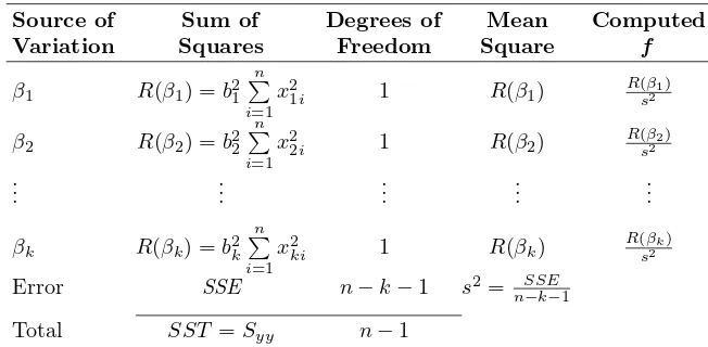
Table 12.4: Analysis of Variance for Orthogonal Variables
Source of Sum of Degrees of Mean Computed
Variation Squares Freedom Square f
β1 R(β1) =b21
n i=1
x2
1i 1 R(β1) R(β
1)
s2
β2 R(β2) =b22
n i=1
x2
2i 1 R(β2) R(sβ22) ..
. ... ... ... ...
βk R(βk) =b2k n i=1
x2
ki 1 R(βk) R(sβ2k)
Error SSE n−k−1 s2= SSE
n−k−1
Total SST =Syy n−1
Example 12.8: Suppose that a scientist takes experimental data on the radius of a propellant grain
Yas a function of powder temperaturex1, extrusion ratex2, and die temperature x3. Fit a linear regression model for predicting grain radius, and determine the
effectiveness of each variable in the model. The data are given in Table 12.5.
Table 12.5: Data for Example 12.8
Powder Extrusion Die
Grain Radius Temperature Rate Temperature 82
93 114 124 111 129 157 164
150 (−1) 190 (+1) 150 (−1) 150 (−1) 190 (+1) 190 (+1) 150 (−1) 190 (+1)
12 (−1) 12 (−1) 24 (+1) 12 (−1) 24 (+1) 12 (−1) 24 (+1) 24 (+1)
220 (−1) 220 (−1) 220 (−1) 250 (+1) 220 (−1) 250 (+1) 250 (+1) 250 (+1)
Solution:Note that each variable is controlled at two levels, and the experiment is composed of the eight possible combinations. The data on the independent variables are coded for convenience by means of the following formulas:
x1=
powder temperature−170
20 ,
x2=
extrusion rate−18
6 ,
x3=
die temperature−235
15 .
The resulting levels of x1, x2, andx3 take on the values−1 and +1 as indicated
orthogonal-470 Chapter 12 Multiple Linear Regression and Certain Nonlinear Regression Models
ity that we want to illustrate here. (A more thorough treatment of this type of experimental layout appears in Chapter 15.) TheXmatrix is
X=
and the orthogonality conditions are readily verified. We can now compute coefficients
b0=1 so in terms of the coded variables, the prediction equation is
ˆ
y= 121.75 + 2.5x1+ 14.75x2+ 21.75x3.
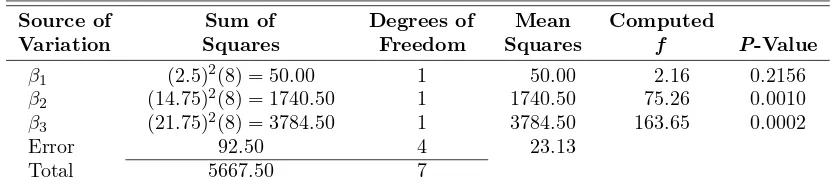
The analysis of variance in Table 12.6 shows independent contributions toSSRfor each variable. The results, when compared to thef0.05(1,4) critical point of 7.71,
indicate thatx1does not contribute significantly at the 0.05 level, whereas variables x2 and x3 are significant. In this example, the estimate for σ2 is 23.1250. As for
the single independent variable case, it should be pointed out that this estimate does not solely contain experimental error variation unless the postulated model is correct. Otherwise, the estimate is “contaminated” by lack of fit in addition to pure error, and the lack of fit can be separated out only if we obtain multiple experimental observations for the various (x1, x2, x3) combinations.
Table 12.6: Analysis of Variance for Grain Radius Data
Source of Sum of Degrees of Mean Computed
Variation Squares Freedom Squares f P-Value
β1
Sincex1 is not significant, it can simply be eliminated from the model without
altering the effects of the other variables. Note that x2 and x3 both impact the
grain radius in a positive fashion, with x3being the more important factor based
/ /
Exercises 471
Exercises
12.31 Compute and interpret the coefficient of multi-ple determination for the variables of Exercise 12.1 on page 450.
12.32 Test whether the regression explained by the model in Exercise 12.1 on page 450 is significant at the 0.01 level of significance.
12.33 Test whether the regression explained by the model in Exercise 12.5 on page 450 is significant at the 0.01 level of significance.
12.34 For the model of Exercise 12.5 on page 450, test the hypothesis
H0: β1=β2= 0,
H1: β1 andβ2 are not both zero.
12.35 Repeat Exercise 12.17 on page 461 using an
F-statistic.
12.36 A small experiment was conducted to fit a mul-tiple regression equation relating the yieldyto temper-ature x1, reaction time x2, and concentration of one
of the reactants x3. Two levels of each variable were
chosen, and measurements corresponding to the coded independent variables were recorded as follows:
y x1 x2 x3
(a) Using the coded variables, estimate the multiple linear regression equation
μY|x1,x2,x3 =β0+β1x1+β2x2+β3x3.
(b) Partition SSR, the regression sum of squares, into three single-degree-of-freedom components at-tributable tox1,x2, andx3, respectively. Show an
analysis-of-variance table, indicating significance tests on each variable.
12.37 Consider the electric power data of Exercise 12.5 on page 450. Test H0:β1 =β2 = 0, making use
ofR(β1, β2|β3, β4). Give aP-value, and draw
conclu-sions.
12.38 Consider the data for Exercise 12.36. Compute the following:
R(β1 |β0), R(β1 |β0, β2, β3),
R(β2 |β0, β1), R(β2 |β0, β1, β3),
R(β3 |β0, β1, β2), R(β1, β2 |β3).
Comment.
12.39 Consider the data of Exercise 11.55 on page 437. Fit a regression model using weight and drive ratio as explanatory variables. Compare this model with the SLR (simple linear regression) model using weight alone. Use R2, R2adj, and any t-statistics (or
F-statistics) you may need to compare the SLR with the multiple regression model.
12.40 Consider Example 12.4. Figure 12.1 on page 459 displays aSASprintout of an analysis of the model containing variables x1, x2, and x3. Focus on the
confidence interval of the mean response μY at the (x1, x2, x3) locations representing the 13 data points.
Consider an item in the printout indicated by C.V. This is thecoefficient of variation, which is defined by
C.V. = s ¯
y·100,
wheres=√s2is theroot mean squared error. The
coefficient of variation is often used as yet another crite-rion for comparing competing models. It is a scale-free quantity which expresses the estimate ofσ, namely s, as a percent of the average response ¯y. In competition for the “best” among a group of competing models, one strives for the model with a small value of C.V. Do a regression analysis of the data set shown in Example 12.4 but eliminate x3. Compare the full (x1, x2, x3)
model with the restricted (x1, x2) model and focus on
two criteria: (i) C.V.; (ii) the widths of the confidence intervals onμY. For the second criterion you may want to use the average width. Comment.
12.41 Consider Example 12.3 on page 447. Compare the two competing models.
First order: yi=β0+β1x1i+β2x2i+ǫi,
Second order: yi=β0+β1x1i+β2x2i
+β11x21i+β22x22i+β12x1ix2i+ǫi.
UseR2adj in your comparison. Test H0: β11 =β22 =
β12= 0. In addition, use the C.V. discussed in Exercise
12.42 In Example 12.8, a case is made for eliminat-ing x1, powder temperature, from the model since the
P-value based on the F-test is 0.2156 while P-values forx2 andx3 are near zero.
(a) Reduce the model by eliminatingx1, thereby
pro-ducing a full and a restricted (or reduced) model, and compare them on the basis ofR2adj.
(b) Compare the full and restricted models using the width of the 95% prediction intervals on a new ob-servation. The better of the two models would be that with the tightened prediction intervals. Use the average of the width of the prediction intervals.
12.43 Consider the data of Exercise 12.13 on page 452. Can the response, wear, be explained adequately by a single variable (either viscosity or load) in an SLR rather than with the full two-variable regression? Jus-tify your answer thoroughly through tests of hypothe-ses as well as comparison of the three competing models.
12.44 For the data set given in Exericise 12.16 on page 453, can the response be explained adequately by any two regressor variables? Discuss.
12.8
Categorical or Indicator Variables
An extremely important special-case application of multiple linear regression oc-curs when one or more of the regressor variables are categorical, indicator, or dummy variables. In a chemical process, the engineer may wish to model the process yield against regressors such as process temperature and reaction time. However, there is interest in using two different catalysts and somehow including “the catalyst” in the model. The catalyst effect cannot be measured on a contin-uum and is hence a categorical variable. An analyst may wish to model the price of homes against regressors that include square feet of living space x1, the land
acreage x2, and age of the house x3. These regressors are clearly continuous in
nature. However, it is clear that cost of homes may vary substantially from one area of the country to another. If data are collected on homes in the east, mid-west, south, and mid-west, we have an indicator variable withfour categories. In the chemical process example, if two catalysts are used, we have an indicator variable with two categories. In a biomedical example in which a drug is to be compared to a placebo, all subjects are evaluated on several continuous measurements such as age, blood pressure, and so on, as well as gender, which of course is categori-cal with two categories. So, included along with the continuous variables are two indicator variables: treatment with two categories (active drug and placebo) and gender with two categories (male and female).
Model with Categorical Variables
Let us use the chemical processing example to illustrate how indicator variables are involved in the model. Suppose y = yield and x1 = temperature and x2 =
reaction time. Now let us denote the indicator variable byz. Letz= 0 for catalyst 1 and z= 1 for catalyst 2. The assignment of the (0,1) indicator to the catalyst is arbitrary. As a result, the model becomes
yi=β0+β1x1i+β2x2i+β3zi+ǫi, i= 1,2, . . . , n.
Three Categories
12.8 Categorical or Indicator Variables 473
includetworegressors, say z1and z2, where the (0,1) assignment is as follows:
z1 z2
⎡
⎣10 01
0 0
⎤ ⎦,
where 0and1are vectors of 0’s and 1’s, respectively. In other words, if there are
ℓcategories, the model includesℓ−1 actual model terms.
It may be instructive to look at a graphical representation of the model with three categories. For the sake of simplicity, let us assume a single continuous variablex. As a result, the model is given by
yi=β0+β1xi+β2z1i+β3z2i+ǫi.
Thus, Figure 12.2 reflects the nature of the model. The following are model ex-pressions for the three categories.
E(Y) = (β0+β2) +β1x, category 1, E(Y) = (β0+β3) +β1x, category 2, E(Y) =β0+β1x, category 3.
As a result, the model involving categorical variables essentially involves achange in the interceptas we change from one category to another. Here of course we are assuming that thecoefficients of continuous variables remain the same across the categories.
x y
Category 3 Category 2 Category 1
Figure 12.2: Case of three categories.
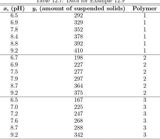
Example 12.9: Consider the data in Table 12.7. The response y is the amount of suspended solids in a coal cleansing system. The variable x is the pH of the system. Three different polymers are used in the system. Thus, “polymer” is categorical with three categories and hence produces two model terms. The model is given by
Here we have
z1=
1, for polymer 1,
0, otherwise, and z2=
1, for polymer 2, 0, otherwise.
From the analysis in Figure 12.3, the following conclusions are drawn. The coefficientb1for pH is the estimate of thecommon slopethat is assumed in the
regression analysis. All model terms are statistically significant. Thus, pH and the nature of the polymer have an impact on the amount of cleansing. The signs and magnitudes of the coefficients ofz1andz2indicate that polymer 1 is most effective
(producing higher suspended solids) for cleansing, followed by polymer 2. Polymer 3 is least effective.
Table 12.7: Data for Example 12.9
x, (pH) y, (amount of suspended solids) Polymer
6.5 292 1
6.9 329 1
7.8 352 1
8.4 378 1
8.8 392 1
9.2 410 1
6.7 198 2
6.9 227 2
7.5 277 2
7.9 297 2
8.7 364 2
9.2 375 2
6.5 167 3
7.0 225 3
7.2 247 3
7.6 268 3
8.7 288 3
9.2 342 3
Slope May Vary with Indicator Categories
In the discussion given here, we have assumed that the indicator variable model terms enter the model in an additive fashion. This suggests that the slopes, as in Figure 12.2, are constant across categories. Obviously, this is not always going to be the case. We can account for the possibility of varying slopes and indeed test for this condition of parallelismby including product orinteractionterms between indicator terms and continuous variables. For example, suppose a model with one continuous regressor and an indicator variable with two levels is chosen. The model is given by
12.8 Categorical or Indicator Variables 475
Sum of
Source DF Squares Mean Square F Value Pr > F Model 3 80181.73127 26727.24376 73.68 <.0001 Error 14 5078.71318 362.76523
Corrected Total 17 85260.44444
R-Square Coeff Var Root MSE y Mean 0.940433 6.316049 19.04640 301.5556
Standard Parameter Estimate Error t Value Pr > |t| Intercept -161.8973333 37.43315576 -4.32 0.0007 x 54.2940260 4.75541126 11.42 <.0001 z1 89.9980606 11.05228237 8.14 <.0001 z2 27.1656970 11.01042883 2.47 0.0271
Figure 12.3: SASprintout for Example 12.9.
This model suggests that for category l (z= 1),
E(y) = (β0+β2) + (β1+β3)x,
while for category 2 (z= 0),
E(y) =β0+β1x.
Thus, we allow for varying intercepts and slopes for the two categories. Figure 12.4 displays the regression lines with varying slopes for the two categories.
y
x
Category 1: slope =β1
Category 2: slope =β1
β3
β0
β2
+
Figure 12.4: Nonparallelism in categorical variables.
In this case,β0,β1, andβ2are positive whileβ3is negative with|β3|< β1.
Ob-viously, if the interaction coefficientβ3is insignificant, we are back to the common
Exercises
12.45 A study was done to assess the cost effective-ness of driving a four-door sedan instead of a van or an SUV (sports utility vehicle). The continuous variables are odometer reading and octane of the gasoline used. The response variable is miles per gallon. The data are presented here.
MPG Car Type Odometer Octane
34.5 sedan 75,000 87.5 33.3 sedan 60,000 87.5 30.4 sedan 88,000 78.0 32.8 sedan 15,000 78.0 35.0 sedan 25,000 90.0 29.0 sedan 35,000 78.0 32.5 sedan 102,000 90.0 29.6 sedan 98,000 87.5 16.8 van 56,000 87.5 19.2 van 72,000 90.0 22.6 van 14,500 87.5 24.4 van 22,000 90.0 20.7 van 66,500 78.0 25.1 van 35,000 90.0 18.8 van 97,500 87.5 15.8 van 65,500 78.0 17.4 van 42,000 78.0 15.6 SUV 65,000 78.0 17.3 SUV 55,500 87.5 20.8 SUV 26,500 87.5 22.2 SUV 11,500 90.0 16.5 SUV 38,000 78.0 21.3 SUV 77,500 90.0 20.7 SUV 19,500 78.0 24.1 SUV 87,000 90.0 (a) Fit a linear regression model including two
indica-tor variables. Use (0,0) to denote the four-door sedan.
(b) Which type of vehicle appears to get the best gas mileage?
(c) Discuss the difference between a van and an SUV in terms of gas mileage.
12.46 A study was done to determine whether the gender of the credit card holder was an important fac-tor in generating profit for a certain credit card com-pany. The variables considered were income, the num-ber of family memnum-bers, and the gender of the card holder. The data are as follows:
Family Profit Income Gender Members
157
(a) Fit a linear regression model using the variables available. Based on the fitted model, would the company prefer male or female customers? (b) Would you say that income was an important
fac-tor in explaining the variability in profit?
12.9
Sequential Methods for Model Selection
At times, the significance tests outlined in Section 12.6 are quite adequate for determining which variables should be used in the final regression model. These tests are certainly effective if the experiment can be planned and the variables are orthogonal to each other. Even if the variables are not orthogonal, the individual