Probability & Statistics for
Engineers & Scientists
N I N T H
E D I T I O N
Ronald E. Walpole
Roanoke College
Raymond H. Myers
Virginia Tech
Sharon L. Myers
Radford University
Keying Ye
University of Texas at San Antonio
Fundamental Sampling
Distributions and Data Descriptions
8.1
Random Sampling
The outcome of a statistical experiment may be recorded either as a numerical value or as a descriptive representation. When a pair of dice is tossed and the total is the outcome of interest, we record a numerical value. However, if the students of a certain school are given blood tests and the type of blood is of interest, then a descriptive representation might be more useful. A person’s blood can be classified in 8 ways: AB, A, B, or O, each with a plus or minus sign, depending on the presence or absence of the Rh antigen.
In this chapter, we focus on sampling from distributions or populations and study such important quantities as the sample meanand sample variance, which will be of vital importance in future chapters. In addition, we attempt to give the reader an introduction to the role that the sample mean and variance will play in statistical inference in later chapters. The use of modern high-speed computers allows the scientist or engineer to greatly enhance his or her use of formal statistical inference with graphical techniques. Much of the time, formal inference appears quite dry and perhaps even abstract to the practitioner or to the manager who wishes to let statistical analysis be a guide to decision-making.
Populations and Samples
We begin this section by discussing the notions ofpopulations andsamples. Both are mentioned in a broad fashion in Chapter 1. However, much more needs to be presented about them here, particularly in the context of the concept of random variables. The totality of observations with which we are concerned, whether their number be finite or infinite, constitutes what we call apopulation. There was a time when the word population referred to observations obtained from statistical studies about people. Today, statisticians use the term to refer to observations relevant to anything of interest, whether it be groups of people, animals, or all possible outcomes from some complicated biological or engineering system.
Definition 8.1: A population consists of the totality of the observations with which we are concerned.
The number of observations in the population is defined to be the size of the population. If there are 600 students in the school whom we classified according to blood type, we say that we have a population of size 600. The numbers on the cards in a deck, the heights of residents in a certain city, and the lengths of fish in a particular lake are examples of populations with finite size. In each case, the total number of observations is a finite number. The observations obtained by measuring the atmospheric pressure every day, from the past on into the future, or all measurements of the depth of a lake, from any conceivable position, are examples of populations whose sizes are infinite. Some finite populations are so large that in theory we assume them to be infinite. This is true in the case of the population of lifetimes of a certain type of storage battery being manufactured for mass distribution throughout the country.
Each observation in a population is a value of a random variableX having some probability distributionf(x). If one is inspecting items coming off an assembly line for defects, then each observation in the population might be a value 0 or 1 of the Bernoulli random variableX with probability distribution
b(x; 1, p) =pxq1−x, x= 0,1
where 0 indicates a nondefective item and 1 indicates a defective item. Of course, it is assumed thatp, the probability of any item being defective, remains constant from trial to trial. In the blood-type experiment, the random variableX represents the type of blood and is assumed to take on values from 1 to 8. Each student is given one of the values of the discrete random variable. The lives of the storage batteries are values assumed by a continuous random variable having perhaps a normal distribution. When we refer hereafter to a “binomial population,” a “nor-mal population,” or, in general, the “populationf(x),” we shall mean a population whose observations are values of a random variable having a binomial distribution, a normal distribution, or the probability distributionf(x). Hence, the mean and variance of a random variable or probability distribution are also referred to as the mean and variance of the corresponding population.
In the field of statistical inference, statisticians are interested in arriving at con-clusions concerning a population when it is impossible or impractical to observe the entire set of observations that make up the population. For example, in attempting to determine the average length of life of a certain brand of light bulb, it would be impossible to test all such bulbs if we are to have any left to sell. Exorbitant costs can also be a prohibitive factor in studying an entire population. Therefore, we must depend on a subset of observations from the population to help us make inferences concerning that same population. This brings us to consider the notion of sampling.
Definition 8.2: Asampleis a subset of a population.
tempted to choose a sample by selecting the most convenient members of the population. Such a procedure may lead to erroneous inferences concerning the population. Any sampling procedure that produces inferences that consistently overestimate or consistently underestimate some characteristic of the population is said to bebiased. To eliminate any possibility of bias in the sampling procedure, it is desirable to choose arandom samplein the sense that the observations are made independently and at random.
In selecting a random sample of sizenfrom a populationf(x), let us define the random variable Xi, i= 1,2, . . . , n, to represent the ith measurement or sample value that we observe. The random variablesX1, X2, . . . , Xn will then constitute a random sample from the populationf(x) with numerical valuesx1, x2, . . . , xn if the measurements are obtained by repeating the experimentnindependent times under essentially the same conditions. Because of the identical conditions under which the elements of the sample are selected, it is reasonable to assume that then
random variablesX1, X2, . . . , Xnare independent and that each has the same prob-ability distribution f(x). That is, the probability distributions ofX1, X2, . . . , Xn are, respectively, f(x1), f(x2), . . . , f(xn), and their joint probability distribution is f(x1, x2, . . . , xn) = f(x1)f(x2)· · ·f(xn). The concept of a random sample is described formally by the following definition.
Definition 8.3: Let X1, X2, . . . , Xn be n independent random variables, each having the same probability distributionf(x). DefineX1, X2, . . . , Xn to be arandom sampleof sizenfrom the populationf(x) and write its joint probability distribution as
f(x1, x2, . . . , xn) =f(x1)f(x2)· · ·f(xn).
If one makes a random selection ofn= 8 storage batteries from a manufacturing process that has maintained the same specification throughout and records the length of life for each battery, with the first measurementx1 being a value ofX1, the second measurement x2 a value of X2, and so forth, then x1, x2, . . . , x8 are the values of the random sample X1, X2, . . . , X8. If we assume the population of battery lives to be normal, the possible values of any Xi, i = 1,2, . . . ,8, will be precisely the same as those in the original population, and henceXi has the same identical normal distribution asX.
8.2
Some Important Statistics
Our main purpose in selecting random samples is to elicit information about the unknown population parameters. Suppose, for example, that we wish to arrive at a conclusion concerning the proportion of coffee-drinkers in the United States who prefer a certain brand of coffee. It would be impossible to question every coffee-drinking American in order to compute the value of the parameter prepresenting the population proportion. Instead, a large random sample is selected and the proportion ˆpof people in this sample favoring the brand of coffee in question is calculated. The value ˆp is now used to make an inference concerning the true proportion p.
random samples are possible from the same population, we would expect ˆpto vary somewhat from sample to sample. That is, ˆpis a value of a random variable that we represent by P. Such a random variable is called a statistic.
Definition 8.4: Any function of the random variables constituting a random sample is called a statistic.
Location Measures of a Sample: The Sample Mean, Median, and Mode
In Chapter 4 we introduced the two parametersµandσ2, which measure the center of location and the variability of a probability distribution. These are constant population parameters and are in no way affected or influenced by the observations of a random sample. We shall, however, define some important statistics that describe corresponding measures of a random sample. The most commonly used statistics for measuring the center of a set of data, arranged in order of magnitude, are themean,median, andmode. Although the first two of these statistics were defined in Chapter 1, we repeat the definitions here. LetX1, X2, . . . , Xn represent
nrandom variables. (a) Sample mean:
¯
X = 1
n
n
i=1
Xi.
Note that the statistic ¯X assumes the value ¯x = 1n n
i=1
xi when X1 assumes the
valuex1,X2assumes the valuex2, and so forth. The termsample meanis applied to both the statistic ¯X and its computed value ¯x.
(b) Sample median:
˜
x=
x(n+1)/2, ifnis odd, 1
2(xn/2+xn/2+1), ifnis even.
The sample median is also a location measure that shows the middle value of the sample. Examples for both the sample mean and the sample median can be found in Section 1.3. The sample mode is defined as follows.
(c) The sample mode is the value of the sample that occurs most often.
Example 8.1: Suppose a data set consists of the following observations:
0.32 0.53 0.28 0.37 0.47 0.43 0.36 0.42 0.38 0.43.
Variability Measures of a Sample: The Sample Variance, Standard Deviation,
and Range
The variability in a sample displays how the observations spread out from the average. The reader is referred to Chapter 1 for more discussion. It is possible to have two sets of observations with the same mean or median that differ considerably in the variability of their measurements about the average.
Consider the following measurements, in liters, for two samples of orange juice bottled by companiesAandB:
SampleA 0.97 1.00 0.94 1.03 1.06 SampleB 1.06 1.01 0.88 0.91 1.14
Both samples have the same mean, 1.00 liter. It is obvious that company A
bottles orange juice with a more uniform content than company B. We say that the variability, or the dispersion, of the observations from the average is less for sampleAthan for sampleB. Therefore, in buying orange juice, we would feel more confident that the bottle we select will be close to the advertised average if we buy from companyA.
In Chapter 1 we introduced several measures of sample variability, including the sample variance, sample standard deviation, and sample range. In this chapter, we will focus mainly on the sample variance. Again, let X1, . . . , Xn representnrandom variables.
(a) Sample variance:
S2= 1
n−1 n
i=1
(Xi−X¯)2. (8.2.1)
The computed value of S2 for a given sample is denoted by s2. Note that
S2 is essentially defined to be the average of the squares of the deviations of the observations from their mean. The reason for usingn−1 as a divisor rather than the more obvious choicenwill become apparent in Chapter 9.
Example 8.2: A comparison of coffee prices at 4 randomly selected grocery stores in San Diego showed increases from the previous month of 12, 15, 17, and 20 cents for a 1-pound bag. Find the variance of this random sample of price increases.
Solution:Calculating the sample mean, we get
¯
x=12 + 15 + 17 + 20
4 = 16 cents.
Therefore,
s2= 1 3
4
i=1
(xi−16)2=
(12−16)2+ (15−16)2+ (17−16)2+ (20−16)2 3
= (−4)
2+ (−1)2+ (1)2+ (4)2
3 =
34 3 .
230 Chapter 8 Fundamental Sampling Distributions and Data Descriptions
Theorem 8.1: IfS2is the variance of a random sample of sizen, we may write
S2= 1
As in Chapter 1, thesample standard deviationand thesample rangeare defined below.
(b) Sample standard deviation:
S=√S2,
where S2is the sample variance.
LetXmax denote the largest of theXi values andXmin the smallest.
(c) Sample range:
R=Xmax−Xmin.
Example 8.3: Find the variance of the data 3, 4, 5, 6, 6, and 7, representing the number of trout caught by a random sample of 6 fishermen on June 19, 1996, at Lake Muskoka.
Solution:We find that 6
8.1 Define suitable populations from which the fol-lowing samples are selected:
(a) Persons in 200 homes in the city of Richmond are called on the phone and asked to name the candi-date they favor for election to the school board. (b) A coin is tossed 100 times and 34 tails are recorded.
(c) Two hundred pairs of a new type of tennis shoe were tested on the professional tour and, on aver-age, lasted 4 months.
Exercises 231
8.2 The lengths of time, in minutes, that 10 patients waited in a doctor’s office before receiving treatment were recorded as follows: 5, 11, 9, 5, 10, 15, 6, 10, 5, and 10. Treating the data as a random sample, find (a) the mean;
(b) the median; (c) the mode.
8.3 The reaction times for a random sample of 9 sub-jects to a stimulant were recorded as 2.5, 3.6, 3.1, 4.3, 2.9. 2.3, 2.6, 4.1, and 3.4 seconds. Calculate
(a) the mean; (b) the median.
8.4 The number of tickets issued for traffic violations by 8 state troopers during the Memorial Day weekend are 5, 4, 7, 7, 6, 3, 8, and 6.
(a) If these values represent the number of tickets is-sued by a random sample of 8 state troopers from Montgomery County in Virginia, define a suitable population.
(b) If the values represent the number of tickets issued by a random sample of 8 state troopers from South Carolina, define a suitable population.
8.5 The numbers of incorrect answers on a true-false competency test for a random sample of 15 students were recorded as follows: 2, 1, 3, 0, 1, 3, 6, 0, 3, 3, 5, 2, 1, 4, and 2. Find
(a) the mean; (b) the median; (c) the mode.
8.6 Find the mean, median, and mode for the sample whose observations, 15, 7, 8, 95, 19, 12, 8, 22, and 14, represent the number of sick days claimed on 9 fed-eral income tax returns. Which value appears to be the best measure of the center of these data? State reasons for your preference.
8.7 A random sample of employees from a local man-ufacturing plant pledged the following donations, in dollars, to the United Fund: 100, 40, 75, 15, 20, 100, 75, 50, 30, 10, 55, 75, 25, 50, 90, 80, 15, 25, 45, and 100. Calculate
(a) the mean; (b) the mode.
8.8 According to ecology writer Jacqueline Killeen, phosphates contained in household detergents pass right through our sewer systems, causing lakes to turn into swamps that eventually dry up into deserts. The following data show the amount of phosphates per load
of laundry, in grams, for a random sample of various types of detergents used according to the prescribed directions:
For the given phosphate data, find (a) the mean;
(b) the median; (c) the mode.
8.9 Consider the data in Exercise 8.2, find (a) the range;
(b) the standard deviation.
8.10 For the sample of reaction times in Exercise 8.3, calculate
(a) the range;
(b) the variance, using the formula of form (8.2.1).
8.11 For the data of Exercise 8.5, calculate the vari-ance using the formula
(a) of form (8.2.1); (b) in Theorem 8.1.
8.12 The tar contents of 8 brands of cigarettes se-lected at random from the latest list released by the Federal Trade Commission are as follows: 7.3, 8.6, 10.4, 16.1, 12.2, 15.1, 14.5, and 9.3 milligrams. Calculate (a) the mean;
(b) the variance.
8.13 The grade-point averages of 20 college seniors selected at random from a graduating class are as fol-lows:
value in the sample.
(b) Show that the sample variance becomes c2 times its original value if each observation in the sample is multiplied byc.
8.15 Verify that the variance of the sample 4, 9, 3, 6, 4, and 7 is 5.1, and using this fact, along with the results of Exercise 8.14, find
(a) the variance of the sample 12, 27, 9, 18, 12, and 21; (b) the variance of the sample 9, 14, 8, 11, 9, and 12.
8.16 In the 2004-05 football season, University of Southern California had the following score differences for the 13 games it played.
11 49 32 3 6 38 38 30 8 40 31 5 36
Find
(a) the mean score difference; (b) the median score difference.
8.3
Sampling Distributions
The field of statistical inference is basically concerned with generalizations and predictions. For example, we might claim, based on the opinions of several people interviewed on the street, that in a forthcoming election 60% of the eligible voters in the city of Detroit favor a certain candidate. In this case, we are dealing with a random sample of opinions from a very large finite population. As a second il-lustration we might state that the average cost to build a residence in Charleston, South Carolina, is between $330,000 and $335,000, based on the estimates of 3 contractors selected at random from the 30 now building in this city. The popu-lation being sampled here is again finite but very small. Finally, let us consider a soft-drink machine designed to dispense, on average, 240 milliliters per drink. A company official who computes the mean of 40 drinks obtains ¯x= 236 milliliters and, on the basis of this value, decides that the machine is still dispensing drinks with an average content of µ = 240 milliliters. The 40 drinks represent a sam-ple from the infinite population of possible drinks that will be dispensed by this machine.
Inference about the Population from Sample Information
In each of the examples above, we computed a statistic from a sample selected from the population, and from this statistic we made various statements concerning the values of population parameters that may or may not be true. The company official made the decision that the soft-drink machine dispenses drinks with an average content of 240 milliliters, even though the sample mean was 236 milliliters, because he knows from sampling theory that, if µ = 240 milliliters, such a sample value could easily occur. In fact, if he ran similar tests, say every hour, he would expect the values of the statistic ¯xto fluctuate above and belowµ= 240 milliliters. Only when the value of ¯xis substantially different from 240 milliliters will the company official initiate action to adjust the machine.
Since a statistic is a random variable that depends only on the observed sample, it must have a probability distribution.
Definition 8.5: The probability distribution of a statistic is called asampling distribution.
remainder of this chapter we study several of the important sampling distribu-tions of frequently used statistics. Applicadistribu-tions of these sampling distribudistribu-tions to problems of statistical inference are considered throughout most of the remaining chapters. The probability distribution of ¯X is called thesampling distribution of the mean.
What Is the Sampling Distribution of
X
¯
?
We should view the sampling distributions of ¯X and S2 as the mechanisms from which we will be able to make inferences on the parameters µand σ2. The sam-pling distribution of ¯X with sample size n is the distribution that results when anexperiment is conducted over and over(always with sample sizen)and the many values of X¯ result. This sampling distribution, then, describes the variability of sample averages around the population mean µ. In the case of the soft-drink machine, knowledge of the sampling distribution of ¯X arms the analyst with the knowledge of a “typical” discrepancy between an observed ¯xvalue and trueµ. The same principle applies in the case of the distribution ofS2. The sam-pling distribution produces information about the variability of s2 values around
σ2 in repeated experiments.
8.4
Sampling Distribution of Means and the Central Limit
Theorem
The first important sampling distribution to be considered is that of the mean ¯
X. Suppose that a random sample of n observations is taken from a normal population with meanµand varianceσ2. Each observation X
i, i= 1,2, . . . , n, of the random sample will then have the same normal distribution as the population being sampled. Hence, by the reproductive property of the normal distribution established in Theorem 7.11, we conclude that
¯
X = 1
n(X1+X2+· · ·+Xn)
has a normal distribution with mean
µX¯ = 1
n(µ+µ+· · ·+µ
nterms
) =µand varianceσX2¯ = 1
n2(σ
2+σ2+
· · ·+σ2
n terms
) =σ 2
n.
The Central Limit Theorem
Theorem 8.2: Central Limit Theorem: If ¯X is the mean of a random sample of size ntaken from a population with meanµand finite varianceσ2, then the limiting form of the distribution of
Z =X¯−µ
σ/√n,
asn→ ∞, is the standard normal distributionn(z; 0,1).
The normal approximation for ¯X will generally be good if n ≥ 30, provided the population distribution is not terribly skewed. Ifn <30, the approximation is good only if the population is not too different from a normal distribution and, as stated above, if the population is known to be normal, the sampling distribution of ¯X will follow a normal distribution exactly, no matter how small the size of the samples.
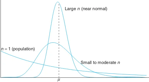
The sample sizen = 30 is a guideline to use for the Central Limit Theorem. However, as the statement of the theorem implies, the presumption of normality on the distribution of ¯X becomes more accurate asngrows larger. In fact, Figure 8.1 illustrates how the theorem works. It shows how the distribution of ¯X becomes closer to normal as ngrows larger, beginning with the clearly nonsymmetric dis-tribution of an individual observation (n= 1). It also illustrates that the mean of
¯
X remainsµfor any sample size and the variance of ¯X gets smaller asnincreases.
µ
Large n (near normal)
Small to moderate n n=1 (population)
Figure 8.1: Illustration of the Central Limit Theorem (distribution of ¯X forn= 1, moderate n, and largen).
Example 8.4: An electrical firm manufactures light bulbs that have a length of life that is ap-proximately normally distributed, with mean equal to 800 hours and a standard deviation of 40 hours. Find the probability that a random sample of 16 bulbs will have an average life of less than 775 hours.
Solution:The sampling distribution of ¯X will be approximately normal, withµX¯ = 800 and
region in Figure 8.2.
x
775 800
σx=10
Figure 8.2: Area for Example 8.4.
Corresponding to ¯x= 775, we find that
z=775−800
10 =−2.5, and therefore
P( ¯X <775) =P(Z <−2.5) = 0.0062.
Inferences on the Population Mean
One very important application of the Central Limit Theorem is the determination of reasonable values of the population meanµ. Topics such as hypothesis testing, estimation, quality control, and many others make use of the Central Limit Theo-rem. The following example illustrates the use of the Central Limit Theorem with regard to its relationship with µ, the mean of the population, although the formal application to the foregoing topics is relegated to future chapters.
In the following case study, an illustration is given which draws an inference that makes use of the sampling distribution of ¯X. In this simple illustration, µ
and σ are both known. The Central Limit Theorem and the general notion of sampling distributions are often used to produce evidence about some important aspect of a distribution such as a parameter of the distribution. In the case of the Central Limit Theorem, the parameter of interest is the mean µ. The inference made concerningµmay take one of many forms. Often there is a desire on the part of the analyst that the data (in the form of ¯x) support (or not) some predetermined conjecture concerning the value ofµ. The use of what we know about the sampling distribution can contribute to answering this type of question. In the following case study, the concept of hypothesis testing leads to a formal objective that we will highlight in future chapters.
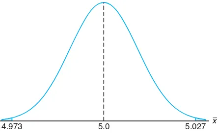
parts having a mean diameter of 5.0 millimeters. The engineer involved conjec-tures that the population mean is 5.0 millimeters. An experiment is conducted in which 100 parts produced by the process are selected randomly and the diameter measured on each. It is known that the population standard deviation is σ= 0.1 millimeter. The experiment indicates a sample average diameter of ¯x= 5.027 mil-limeters. Does this sample information appear to support or refute the engineer’s conjecture?
Solution:This example reflects the kind of problem often posed and solved with hypothesis testing machinery introduced in future chapters. We will not use the formality associated with hypothesis testing here, but we will illustrate the principles and logic used.
Whether the data support or refute the conjecture depends on the probability that data similar to those obtained in this experiment (¯x = 5.027) can readily occur when in fact µ = 5.0 (Figure 8.3). In other words, how likely is it that one can obtain ¯x ≥ 5.027 with n = 100 if the population mean is µ = 5.0? If this probability suggests that ¯x= 5.027 is not unreasonable, the conjecture is not refuted. If the probability is quite low, one can certainly argue that the data do not support the conjecture that µ= 5.0. The probability that we choose to compute is given byP(|X¯ −5| ≥0.027).
x
4.973 5.0 5.027
Figure 8.3: Area for Case Study 8.1.
In other words, if the meanµ is 5, what is the chance that ¯X will deviate by as much as 0.027 millimeter?
P(|X¯−5| ≥0.027) =P( ¯X−5≥0.027) +P( ¯X−5≤ −0.027)
= 2P
¯
X−5
0.1/√100 ≥2.7
.
Here we are simply standardizing ¯X according to the Central Limit Theorem. If the conjectureµ= 5.0 is true, X¯−5
0.1/√100 should followN(0,1). Thus,
2P
¯
X−5
0.1/√100 ≥2.7
Therefore, one would experience by chance that an ¯xwould be 0.027 millimeter from the mean in only 7 in 1000 experiments. As a result, this experiment with ¯
x= 5.027 certainly does not give supporting evidence to the conjecture thatµ= 5.0. In fact, it strongly refutes the conjecture!
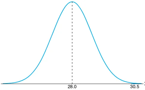
Example 8.5: Traveling between two campuses of a university in a city via shuttle bus takes, on average, 28 minutes with a standard deviation of 5 minutes. In a given week, a bus transported passengers 40 times. What is the probability that the average transport time was more than 30 minutes? Assume the mean time is measured to the nearest minute.
Solution:In this case, µ= 28 andσ= 3. We need to calculate the probability P( ¯X >30) with n = 40. Since the time is measured on a continuous scale to the nearest minute, an ¯xgreater than 30 is equivalent to ¯x≥30.5. Hence,
P( ¯X >30) =P
X¯
−28 5/√40 ≥
30.5−28 5/√40
=P(Z ≥3.16) = 0.0008.
There is only a slight chance that the average time of one bus trip will exceed 30 minutes. An illustrative graph is shown in Figure 8.4.
x
30.5 28.0
Figure 8.4: Area for Example 8.5.
Sampling Distribution of the Difference between Two Means
The illustration in Case Study 8.1 deals with notions of statistical inference on a single mean µ. The engineer was interested in supporting a conjecture regarding a single population mean. A far more important application involves two popula-tions. A scientist or engineer may be interested in a comparative experiment in which two manufacturing methods, 1 and 2, are to be compared. The basis for that comparison is µ1−µ2, the difference in the population means.
Suppose that we have two populations, the first with mean µ1 and variance
σ2
the second population, independent of the sample from the first population. What can we say about the sampling distribution of the difference ¯X1−X¯2for repeated samples of size n1 and n2? According to Theorem 8.2, the variables ¯X1 and ¯X2 are both approximately normally distributed with meansµ1andµ2 and variances
σ12/n1andσ22/n2, respectively. This approximation improves asn1andn2increase. By choosing independent samples from the two populations we ensure that the variables ¯X1 and ¯X2 will be independent, and then using Theorem 7.11, with
a1 = 1 and a2 = −1, we can conclude that ¯X1−X¯2 is approximately normally
The Central Limit Theorem can be easily extended to the two-sample, two-population case.
Theorem 8.3: If independent samples of size n1 and n2 are drawn at random from two popu-lations, discrete or continuous, with meansµ1 and µ2 and variances σ12 and σ22, respectively, then the sampling distribution of the differences of means, ¯X1−X¯2, is approximately normally distributed with mean and variance given by
µX¯1
is approximately a standard normal variable.
If both n1 and n2 are greater than or equal to 30, the normal approximation for the distribution of ¯X1−X¯2 is very good when the underlying distributions are not too far away from normal. However, even when n1 andn2 are less than 30, the normal approximation is reasonably good except when the populations are decidedly nonnormal. Of course, if both populations are normal, then ¯X1−X¯2has a normal distribution no matter what the sizes ofn1 andn2 are.
The utility of the sampling distribution of the difference between two sample averages is very similar to that described in Case Study 8.1 on page 235 for the case of a single mean. Case Study 8.2 that follows focuses on the use of the difference between two sample means to support (or not) the conjecture that two population means are the same.
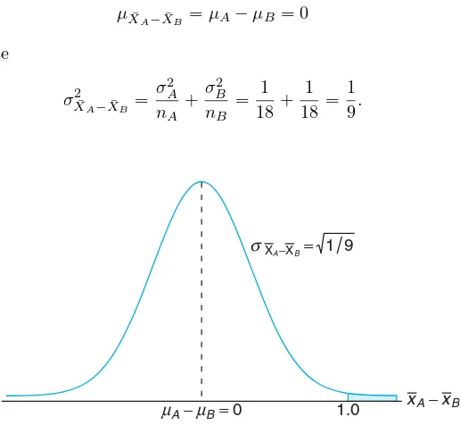
Assuming that the mean drying time is equal for the two types of paint, find
P( ¯XA−X¯B>1.0), where ¯XAand ¯XBare average drying times for samples of size
nA=nB= 18.
Solution: From the sampling distribution of ¯XA−X¯B, we know that the distribution is approximately normal with mean
µX¯A−X¯B =µA−µB= 0
and variance
σ2X¯A−X¯B =
σ2 A
nA +σ
2 B
nB = 1
18+ 1 18 =
1 9.
xA−xB
µA−µB=0 1.0
σXA−XB= 1 9
Figure 8.5: Area for Case Study 8.2.
The desired probability is given by the shaded region in Figure 8.5. Corre-sponding to the value ¯XA−X¯B = 1.0, we have
z= 1−(µA−µB)
1/9 = 1−0
1/9 = 3.0;
so
P(Z >3.0) = 1−P(Z <3.0) = 1−0.9987 = 0.0013.
What Do We Learn from Case Study 8.2?
that the difference in the two sample averages is as small as, say, 15 minutes. If
µA=µB,
P[( ¯XA−X¯B)>0.25 hour] =P
¯
XA−X¯B−0
1/9 > 3 4
=P
Z > 3
4
= 1−P(Z <0.75) = 1−0.7734 = 0.2266.
Since this probability is not low, one would conclude that a difference in sample means of 15 minutes can happen by chance (i.e., it happens frequently even though
µA=µB). As a result, that type of difference in average drying times certainlyis
not a clear signalthat µA=µB.
As we indicated earlier, a more detailed formalism regarding this and other types of statistical inference (e.g., hypothesis testing) will be supplied in future chapters. The Central Limit Theorem and sampling distributions discussed in the next three sections will also play a vital role.
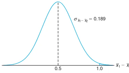
Example 8.6: The television picture tubes of manufacturer Ahave a mean lifetime of 6.5 years and a standard deviation of 0.9 year, while those of manufacturer B have a mean lifetime of 6.0 years and a standard deviation of 0.8 year. What is the probability that a random sample of 36 tubes from manufacturerAwill have a mean lifetime that is at least 1 year more than the mean lifetime of a sample of 49 tubes from manufacturer B?
Solution:We are given the following information:
Population 1 Population 2
µ1= 6.5 µ2= 6.0
σ1= 0.9 σ2= 0.8
n1= 36 n2= 49
If we use Theorem 8.3, the sampling distribution of ¯X1−X¯2 will be approxi-mately normal and will have a mean and standard deviation
µX¯1
−X¯2 = 6.5−6.0 = 0.5 and σX¯1−X¯2 =
"
0.81 36 +
0.64
49 = 0.189.
The probability that the mean lifetime for 36 tubes from manufacturerA will be at least 1 year longer than the mean lifetime for 49 tubes from manufacturerB
is given by the area of the shaded region in Figure 8.6. Corresponding to the value ¯
x1−x¯2= 1.0, we find that
z= 1.0−0.5
0.189 = 2.65,
and hence
Exercises 241
0.5 1.0 x1⫺ x2
x1⫺ x2 ⫽ 0.189
σ
Figure 8.6: Area for Example 8.6.
More on Sampling Distribution of Means—Normal Approximation to
the Binomial Distribution
Section 6.5 presented the normal approximation to the binomial distribution at length. Conditions were given on the parametersnandpfor which the distribution of a binomial random variable can be approximated by the normal distribution. Examples and exercises reflected the importance of the concept of the “normal approximation.” It turns out that the Central Limit Theorem sheds even more light on how and why this approximation works. We certainly know that a binomial random variable is the number X of successes in nindependent trials, where the outcome of each trial is binary. We also illustrated in Chapter 1 that the proportion computed in such an experiment is an average of a set of 0s and 1s. Indeed, while the proportionX/nis an average,X is the sum of this set of 0s and 1s, and both
X and X/n are approximately normal if n is sufficiently large. Of course, from what we learned in Chapter 6, we know that there are conditions onnandpthat affect the quality of the approximation, namelynp≥5 andnq≥5.
Exercises
8.17 If all possible samples of size 16 are drawn from a normal population with mean equal to 50 and stan-dard deviation equal to 5, what is the probability that a sample mean ¯Xwill fall in the interval fromµX¯−1.9σX¯ toµX¯−0.4σX¯? Assume that the sample means can be measured to any degree of accuracy.
8.18 If the standard deviation of the mean for the sampling distribution of random samples of size 36 from a large or infinite population is 2, how large must the sample size become if the standard deviation is to be reduced to 1.2?
8.19 A certain type of thread is manufactured with a mean tensile strength of 78.3 kilograms and a standard deviation of 5.6 kilograms. How is the variance of the
sample mean changed when the sample size is (a) increased from 64 to 196?
(b) decreased from 784 to 49?
8.20 Given the discrete uniform population
f(x) =
1
3, x= 2,4,6, 0, elsewhere,
find the probability that a random sample of size 54, selected with replacement, will yield a sample mean greater than 4.1 but less than 4.4. Assume the means are measured to the nearest tenth.
242 Chapter 8 Fundamental Sampling Distributions and Data Descriptions
a standard deviation of 15 milliliters. Periodically, the machine is checked by taking a sample of 40 drinks and computing the average content. If the mean of the 40 drinks is a value within the intervalµX¯ ±2σX¯, the machine is thought to be operating satisfactorily; oth-erwise, adjustments are made. In Section 8.3, the com-pany official found the mean of 40 drinks to be ¯x= 236 milliliters and concluded that the machine needed no adjustment. Was this a reasonable decision?
8.22 The heights of 1000 students are approximately normally distributed with a mean of 174.5 centimeters and a standard deviation of 6.9 centimeters. Suppose 200 random samples of size 25 are drawn from this pop-ulation and the means recorded to the nearest tenth of a centimeter. Determine
(a) the mean and standard deviation of the sampling distribution of ¯X;
(b) the number of sample means that fall between 172.5 and 175.8 centimeters inclusive;
(c) the number of sample means falling below 172.0 centimeters.
8.23 The random variableX, representing the num-ber of cherries in a cherry puff, has the following prob-ability distribution:
X for random samples of 36 cherry puffs.
(c) Find the probability that the average number of cherries in 36 cherry puffs will be less than 5.5.
8.24 If a certain machine makes electrical resistors having a mean resistance of 40 ohms and a standard deviation of 2 ohms, what is the probability that a random sample of 36 of these resistors will have a com-bined resistance of more than 1458 ohms?
8.25 The average life of a bread-making machine is 7 years, with a standard deviation of 1 year. Assuming that the lives of these machines follow approximately a normal distribution, find
(a) the probability that the mean life of a random sam-ple of 9 such machines falls between 6.4 and 7.2 years;
(b) the value of x to the right of which 15% of the means computed from random samples of size 9 would fall.
8.26 The amount of time that a drive-through bank teller spends on a customer is a random variable with a mean µ = 3.2 minutes and a standard deviation
σ= 1.6 minutes. If a random sample of 64 customers
is observed, find the probability that their mean time at the teller’s window is
(a) at most 2.7 minutes; (b) more than 3.5 minutes;
(c) at least 3.2 minutes but less than 3.4 minutes.
8.27 In a chemical process, the amount of a certain type of impurity in the output is difficult to control and is thus a random variable. Speculation is that the population mean amount of the impurity is 0.20 gram per gram of output. It is known that the standard deviation is 0.1 gram per gram. An experiment is con-ducted to gain more insight regarding the speculation that µ = 0.2. The process is run on a lab scale 50 times and the sample average ¯x turns out to be 0.23 gram per gram. Comment on the speculation that the mean amount of impurity is 0.20 gram per gram. Make use of the Central Limit Theorem in your work.
8.28 A random sample of size 25 is taken from a nor-mal population having a mean of 80 and a standard deviation of 5. A second random sample of size 36 is taken from a different normal population having a mean of 75 and a standard deviation of 3. Find the probability that the sample mean computed from the 25 measurements will exceed the sample mean com-puted from the 36 measurements by at least 3.4 but less than 5.9. Assume the difference of the means to be measured to the nearest tenth.
8.29 The distribution of heights of a certain breed of terrier has a mean of 72 centimeters and a standard de-viation of 10 centimeters, whereas the distribution of heights of a certain breed of poodle has a mean of 28 centimeters with a standard deviation of 5 centimeters. Assuming that the sample means can be measured to any degree of accuracy, find the probability that the sample mean for a random sample of heights of 64 ter-riers exceeds the sample mean for a random sample of heights of 100 poodles by at most 44.2 centimeters.
8.30 The mean score for freshmen on an aptitude test at a certain college is 540, with a standard deviation of 50. Assume the means to be measured to any degree of accuracy. What is the probability that two groups selected at random, consisting of 32 and 50 students, respectively, will differ in their mean scores by (a) more than 20 points?
(b) an amount between 5 and 10 points?
8.31 Consider Case Study 8.2 on page 238. Suppose 18 specimens were used for each type of paint in an experiment and ¯xA−x¯B, the actual difference in mean
drying time, turned out to be 1.0.
two population mean drying times truly are equal? Make use of the result in the solution to Case Study 8.2.
(b) If someone did the experiment 10,000 times un-der the condition that µA = µB, in how many of
those 10,000 experiments would there be a differ-ence ¯xA−x¯B that was as large as (or larger than)
1.0?
8.32 Two different box-filling machines are used to fill cereal boxes on an assembly line. The critical measure-ment influenced by these machines is the weight of the product in the boxes. Engineers are quite certain that the variance of the weight of product isσ2
= 1 ounce. Experiments are conducted using both machines with sample sizes of 36 each. The sample averages for ma-chines A and B are ¯xA = 4.5 ounces and ¯xB = 4.7
ounces. Engineers are surprised that the two sample averages for the filling machines are so different. (a) Use the Central Limit Theorem to determine
P( ¯XB−X¯A≥0.2)
under the condition thatµA=µB.
(b) Do the aforementioned experiments seem to, in any way, strongly support a conjecture that the popu-lation means for the two machines are different? Explain using your answer in (a).
8.33 The chemical benzene is highly toxic to hu-mans. However, it is used in the manufacture of many medicine dyes, leather, and coverings. Government regulations dictate that for any production process in-volving benzene, the water in the output of the process must not exceed 7950 parts per million (ppm) of ben-zene. For a particular process of concern, the water sample was collected by a manufacturer 25 times ran-domly and the sample average ¯xwas 7960 ppm. It is known from historical data that the standard deviation
σis 100 ppm.
(a) What is the probability that the sample average in this experiment would exceed the government limit if the population mean is equal to the limit? Use the Central Limit Theorem.
(b) Is an observed ¯x = 7960 in this experiment firm evidence that the population mean for the process
exceeds the government limit? Answer your ques-tion by computing
P( ¯X≥7960|µ= 7950).
Assume that the distribution of benzene concentra-tion is normal.
8.34 Two alloysAandBare being used to manufac-ture a certain steel product. An experiment needs to be designed to compare the two in terms of maximum load capacity in tons (the maximum weight that can be tolerated without breaking). It is known that the two standard deviations in load capacity are equal at 5 tons each. An experiment is conducted in which 30 specimens of each alloy (A andB) are tested and the results recorded as follows:
¯
xA= 49.5, x¯B= 45.5; x¯A−x¯B= 4.
The manufacturers of alloyA are convinced that this evidence shows conclusively thatµA> µBand strongly
supports the claim that their alloy is superior. Man-ufacturers of alloyB claim that the experiment could easily have given ¯xA−x¯B= 4even ifthe two
popula-tion means are equal. In other words, “the results are inconclusive!”
(a) Make an argument that manufacturers of alloyB
are wrong. Do it by computing
P( ¯XA−X¯B>4|µA=µB).
(b) Do you think these data strongly support alloyA?
8.35 Consider the situation described in Example 8.4 on page 234. Do these results prompt you to question the premise thatµ = 800 hours? Give a probabilis-tic result that indicates howrarean event ¯X ≤775 is whenµ= 800. On the other hand, how rare would it be ifµtruly were, say, 760 hours?
8.36 LetX1, X2, . . . , Xnbe a random sample from a
distribution that can take on only positive values. Use the Central Limit Theorem to produce an argument that if n is sufficiently large, then Y = X1X2· · ·Xn has approximately a lognormal distribution.
8.5
Sampling Distribution of
S
2In the preceding section we learned about the sampling distribution of ¯X. The Central Limit Theorem allowed us to make use of the fact that
¯
tends toward N(0,1) as the sample size grows large. Sampling distributions of important statistics allow us to learn information about parameters. Usually, the parameters are the counterpart to the statistics in question. For example, if an engineer is interested in the population mean resistance of a certain type of resistor, the sampling distribution of ¯X will be exploited once the sample information is gathered. On the other hand, if the variability in resistance is to be studied, clearly the sampling distribution ofS2will be used in learning about the parametric counterpart, the population varianceσ2.
If a random sample of size n is drawn from a normal population with mean
µ and variance σ2, and the sample variance is computed, we obtain a value of the statistic S2. We shall proceed to consider the distribution of the statistic (n−1)S2/σ2.
By the addition and subtraction of the sample mean ¯X, it is easy to see that n
Now, according to Corollary 7.1 on page 222, we know that n
i=1
(Xi−µ)2
σ2
is a chi-squared random variable withndegrees of freedom. We have a chi-squared random variable withndegrees of freedom partitioned into two components. Note that in Section 6.7 we showed that a chi-squared distribution is a special case of a gamma distribution. The second term on the right-hand side is Z2, which is a chi-squared random variable with 1 degree of freedom, and it turns out that (n−1)S2/σ2 is a chi-squared random variable withn−1 degree of freedom. We formalize this in the following theorem.
Theorem 8.4: IfS2is the variance of a random sample of sizentaken from a normal population having the varianceσ2, then the statistic
χ2= (n−1)S
has a chi-squared distribution withv=n−1 degrees of freedom.
formula
χ2=(n−1)s 2
σ2 .
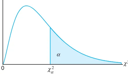
The probability that a random sample produces a χ2 value greater than some specified value is equal to the area under the curve to the right of this value. It is customary to letχ2
αrepresent theχ2 value above which we find an area ofα. This is illustrated by the shaded region in Figure 8.7.
0 χ
χ 2
2 α
α
Figure 8.7: The chi-squared distribution.
Table A.5 gives values ofχ2
α for various values ofαand v. The areas,α, are the column headings; the degrees of freedom,v, are given in the left column; and the table entries are theχ2values. Hence, theχ2 value with 7 degrees of freedom, leaving an area of 0.05 to the right, isχ2
0.05= 14.067. Owing to lack of symmetry, we must also use the tables to findχ2
0.95= 2.167 for v= 7. Exactly 95% of a chi-squared distribution lies betweenχ2
0.975andχ20.025. Aχ2 value falling to the right ofχ20.025is not likely to occur unless our assumed value of
σ2 is too small. Similarly, a χ2 value falling to the left ofχ2
0.975 is unlikely unless our assumed value of σ2 is too large. In other words, it is possible to have a χ2 value to the left of χ2
0.975 or to the right of χ20.025 when σ2 is correct, but if this should occur, it is more probable that the assumed value of σ2is in error.
Example 8.7: A manufacturer of car batteries guarantees that the batteries will last, on average, 3 years with a standard deviation of 1 year. If five of these batteries have lifetimes of 1.9, 2.4, 3.0, 3.5, and 4.2 years, should the manufacturer still be convinced that the batteries have a standard deviation of 1 year? Assume that the battery lifetime follows a normal distribution.
Solution:We first find the sample variance using Theorem 8.1,
s2=(5)(48.26)−(15) 2
(5)(4) = 0.815.
Then
is a value from a chi-squared distribution with 4 degrees of freedom. Since 95% of the χ2 values with 4 degrees of freedom fall between 0.484 and 11.143, the computed value withσ2= 1 is reasonable, and therefore the manufacturer has no reason to suspect that the standard deviation is other than 1 year.
Degrees of Freedom as a Measure of Sample Information
Recall from Corollary 7.1 in Section 7.3 that
n
i=1
(Xi−µ)2
σ2
has a χ2-distribution with n degrees of freedom. Note also Theorem 8.4, which indicates that the random variable
(n−1)S2
σ2 =
n
i=1
(Xi−X¯)2
σ2
has aχ2-distribution withn−1degrees of freedom. The reader may also recall that the term degrees of freedom, used in this identical context, is discussed in Chapter 1.
As we indicated earlier, the proof of Theorem 8.4 will not be given. However, the reader can view Theorem 8.4 as indicating that when µis not known and one considers the distribution of
n
i=1
(Xi−X¯)2
σ2 ,
there is1 less degree of freedom, or a degree of freedom is lost in the estimation of µ (i.e., when µ is replaced by ¯x). In other words, there aren degrees of free-dom, or independentpieces of information, in the random sample from the normal distribution. When the data (the values in the sample) are used to compute the mean, there is 1 less degree of freedom in the information used to estimate σ2.
8.6
t
-Distribution
In Section 8.4, we discussed the utility of the Central Limit Theorem. Its applica-tions revolve around inferences on a population mean or the difference between two population means. Use of the Central Limit Theorem and the normal distribution is certainly helpful in this context. However, it was assumed that the population standard deviation is known. This assumption may not be unreasonable in situ-ations where the engineer is quite familiar with the system or process. However, in many experimental scenarios, knowledge of σ is certainly no more reasonable than knowledge of the population mean µ. Often, in fact, an estimate ofσ must be supplied by the same sample information that produced the sample average ¯x. As a result, a natural statistic to consider to deal with inferences onµis
T = X¯ −µ
sinceS is the sample analog toσ. If the sample size is small, the values ofS2 fluc-tuate considerably from sample to sample (see Exercise 8.43 on page 259) and the distribution ofT deviates appreciably from that of a standard normal distribution. If the sample size is large enough, sayn≥30, the distribution ofT does not differ considerably from the standard normal. However, forn <30, it is useful to deal with the exact distribution ofT. In developing the sampling distribution ofT, we shall assume that our random sample was selected from a normal population. We can then write
T = ( ¯X−µ)/(σ/
√
n)
S2/σ2 =
Z
V /(n−1),
where
Z= X¯ −µ
σ/√n
has the standard normal distribution and
V = (n−1)S 2
σ2
has a chi-squared distribution withv=n−1 degrees of freedom. In sampling from normal populations, we can show that ¯XandS2are independent, and consequently so areZ and V. The following theorem gives the definition of a random variable
T as a function of Z (standard normal) and χ2. For completeness, the density function of the t-distribution is given.
Theorem 8.5: LetZbe a standard normal random variable andV a chi-squared random variable with v degrees of freedom. If Z andV are independent, then the distribution of the random variableT, where
T = Z
V /v,
is given by the density function
h(t) = Γ[(v+ 1)/2] Γ(v/2)√πv
1 +t 2
v
−(v+1)/2
, − ∞< t <∞.
This is known as thet-distributionwithvdegrees of freedom.
Corollary 8.1: Let X1, X2, . . . , Xn be independent random variables that are all normal with meanµand standard deviationσ. Let
¯
X = 1
n
n
i=1
Xi and S2=
1
n−1 n
i=1
(Xi−X¯)2.
Then the random variableT = X¯−µ
S/√n has at-distribution withv=n−1 degrees of freedom.
The probability distribution ofT was first published in 1908 in a paper written by W. S. Gosset. At the time, Gosset was employed by an Irish brewery that prohibited publication of research by members of its staff. To circumvent this re-striction, he published his work secretly under the name “Student.” Consequently, the distribution of T is usually called the Student t-distribution or simply the t -distribution. In deriving the equation of this distribution, Gosset assumed that the samples were selected from a normal population. Although this would seem to be a very restrictive assumption, it can be shown that nonnormal populations possess-ing nearly bell-shaped distributions will still provide values ofT that approximate thet-distribution very closely.
What Does the
t
-Distribution Look Like?
The distribution of T is similar to the distribution of Z in that they both are symmetric about a mean of zero. Both distributions are bell shaped, but the t -distribution is more variable, owing to the fact that the T-values depend on the fluctuations of two quantities, ¯X andS2, whereas theZ-values depend only on the changes in ¯X from sample to sample. The distribution ofT differs from that ofZ
in that the variance ofT depends on the sample sizenand is always greater than 1. Only when the sample sizen→ ∞will the two distributions become the same. In Figure 8.8, we show the relationship between a standard normal distribution (v = ∞) and t-distributions with 2 and 5 degrees of freedom. The percentage points of thet-distribution are given in Table A.4.
⫺2 ⫺1 0 1 2
v ⫽ 2 v⫽ ⬁
v ⫽5
Figure 8.8: The t-distribution curves forv = 2,5, and ∞.
t t1⫺ α⫽ ⫺tα 0 tα
Figure 8.9: Symmetry property (about 0) of the
It is customary to lettαrepresent thet-value above which we find an area equal to α. Hence, the t-value with 10 degrees of freedom leaving an area of 0.025 to the right ist= 2.228. Since thet-distribution is symmetric about a mean of zero, we havet1−α=−tα; that is, thet-value leaving an area of 1−αto the right and
therefore an area ofαto the left is equal to the negativet-value that leaves an area of αin the right tail of the distribution (see Figure 8.9). That is, t0.95 =−t0.05,
t0.99=−t0.01, and so forth.
Example 8.8: Thet-value withv= 14 degrees of freedom that leaves an area of 0.025 to the left, and therefore an area of 0.975 to the right, is
t0.975=−t0.025=−2.145.
Example 8.9: FindP(−t0.025< T < t0.05).
Solution:Since t0.05 leaves an area of 0.05 to the right, and −t0.025 leaves an area of 0.025 to the left, we find a total area of
1−0.05−0.025 = 0.925
between−t0.025 andt0.05. Hence
P(−t0.025< T < t0.05) = 0.925.
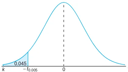
Example 8.10: Find k such that P(k < T < −1.761) = 0.045 for a random sample of size 15 selected from a normal distribution and X−µ
s/√n.
t
0
k −t0.005 0.045
Figure 8.10: Thet-values for Example 8.10.
Solution:From Table A.4 we note that 1.761 corresponds to t0.05 whenv = 14. Therefore,
−t0.05 = −1.761. Since k in the original probability statement is to the left of
−t0.05=−1.761, letk=−tα. Then, from Figure 8.10, we have
0.045 = 0.05−α, orα= 0.005.
Hence, from Table A.4 withv= 14,
Exactly 95% of the values of at-distribution withv=n−1 degrees of freedom lie between−t0.025andt0.025. Of course, there are othert-values that contain 95% of the distribution, such as−t0.02andt0.03, but these values do not appear in Table A.4, and furthermore, the shortest possible interval is obtained by choosingt-values that leave exactly the same area in the two tails of our distribution. At-value that falls below−t0.025or abovet0.025 would tend to make us believe either that a very rare event has taken place or that our assumption aboutµis in error. Should this happen, we shall make the the decision that our assumed value of µ is in error. In fact, a t-value falling below−t0.01 or above t0.01 would provide even stronger evidence that our assumed value of µ is quite unlikely. General procedures for testing claims concerning the value of the parameter µwill be treated in Chapter 10. A preliminary look into the foundation of these procedure is illustrated by the following example.
Example 8.11: A chemical engineer claims that the population mean yield of a certain batch process is 500 grams per milliliter of raw material. To check this claim he samples 25 batches each month. If the computedt-value falls between−t0.05 andt0.05, he is satisfied with this claim. What conclusion should he draw from a sample that has a mean ¯x= 518 grams per milliliter and a sample standard deviation s= 40 grams? Assume the distribution of yields to be approximately normal.
Solution:From Table A.4 we find thatt0.05= 1.711 for 24 degrees of freedom. Therefore, the engineer can be satisfied with his claim if a sample of 25 batches yields a t-value between−1.711 and 1.711. If µ= 500, then
t= 518−500
40/√25 = 2.25,
a value well above 1.711. The probability of obtaining at-value, withv= 24, equal to or greater than 2.25 is approximately 0.02. Ifµ >500, the value oftcomputed from the sample is more reasonable. Hence, the engineer is likely to conclude that the process produces a better product than he thought.
What Is the
t
-Distribution Used For?
The t-distribution is used extensively in problems that deal with inference about the population mean (as illustrated in Example 8.11) or in problems that involve comparative samples (i.e., in cases where one is trying to determine if means from two samples are significantly different). The use of the distribution will be extended in Chapters 9, 10, 11, and 12. The reader should note that use of thet-distribution for the statistic
T = X¯ −µ
S/√n
requires that X1, X2, . . . , Xn be normal. The use of the t-distribution and the sample size consideration do not relate to the Central Limit Theorem. The use of the standard normal distribution rather than T forn≥30 merely implies that
S is a sufficiently good estimator of σ in this case. In chapters that follow the
8.7
F
-Distribution
We have motivated thet-distribution in part by its application to problems in which there is comparative sampling (i.e., a comparison between two sample means). For example, some of our examples in future chapters will take a more formal approach, chemical engineer collects data on two catalysts, biologist collects data on two growth media, or chemist gathers data on two methods of coating material to inhibit corrosion. While it is of interest to let sample information shed light on two population means, it is often the case that a comparison of variability is equally important, if not more so. The F-distribution finds enormous application in comparing sample variances. Applications of the F-distribution are found in problems involving two or more samples.
The statisticF is defined to be the ratio of two independent chi-squared random variables, each divided by its number of degrees of freedom. Hence, we can write
F =U/v1
V /v2
,
whereU andV are independent random variables having chi-squared distributions with v1 andv2 degrees of freedom, respectively. We shall now state the sampling distribution ofF.
Theorem 8.6: LetU andV be two independent random variables having chi-squared distributions with v1 and v2 degrees of freedom, respectively. Then the distribution of the random variableF = U/v1
V /v2 is given by the density function
h(f) =
Γ[(v
1+v2)/2](v1/v2)v1/2 Γ(v1/2)Γ(v2/2)
f(v1/2)−1
(1+v1f /v2)(v1 +v2)/2, f >0,
0, f ≤0.
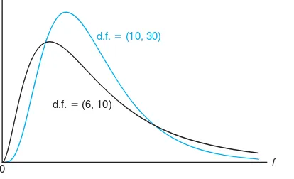
This is known as theF-distributionwithv1 andv2 degrees of freedom (d.f.).
We will make considerable use of the random variableF in future chapters. How-ever, the density function will not be used and is given only for completeness. The curve of theF-distribution depends not only on the two parametersv1andv2but also on the order in which we state them. Once these two values are given, we can identify the curve. TypicalF-distributions are shown in Figure 8.11.
f 0
d.f. ⫽ (6, 10)
d.f. ⫽ (10, 30)
Figure 8.11: TypicalF-distributions.
f
0 f
α
α
Figure 8.12: Illustration of the fα for the F -distribution.
Theorem 8.7: Writingfα(v1, v2) forfαwithv1 andv2 degrees of freedom, we obtain
f1−α(v1, v2) =
1
fα(v2, v1)
.
Thus, thef-value with 6 and 10 degrees of freedom, leaving an area of 0.95 to the right, is
f0.95(6,10) = 1
f0.05(10,6) = 1
4.06 = 0.246.
The
F
-Distribution with Two Sample Variances
Suppose that random samples of size n1 and n2 are selected from two normal populations with variances σ2
1 and σ22, respectively. From Theorem 8.4, we know that
χ21=
(n1−1)S12
σ2 1
andχ22=
(n2−1)S22
σ2 2
are random variables having chi-squared distributions with v1 =n1−1 andv2=
n2−1 degrees of freedom. Furthermore, since the samples are selected at random, we are dealing with independent random variables. Then, using Theorem 8.6 with
χ2
1=U andχ22=V, we obtain the following result.
Theorem 8.8: IfS2
1 andS22 are the variances of independent random samples of size n1 andn2 taken from normal populations with variancesσ2
1 andσ22, respectively, then
F= S
2 1/σ21
S2 2/σ22
=σ 2 2S12
σ2 1S22
What Is the
F
-Distribution Used For?
We answered this question, in part, at the beginning of this section. The F -distribution is used in two-sample situations to draw inferences about the pop-ulation variances. This involves the application of Theorem 8.8. However, the
F-distribution can also be applied to many other types of problems involving sam-ple variances. In fact, theF-distribution is called the variance ratio distribution. As an illustration, consider Case Study 8.2, in which two paints, A and B, were compared with regard to mean drying time. The normal distribution applies nicely (assuming thatσAandσBare known). However, suppose that there are three types of paints to compare, say A, B, and C. We wish to determine if the population means are equivalent. Suppose that important summary information from the experiment is as follows:
Paint Sample Mean Sample Variance Sample Size
A X¯A= 4.5 s2A= 0.20 10
B X¯B= 5.5 s2B= 0.14 10
C X¯C= 6.5 s2C= 0.11 10
The problem centers around whether or not the sample averages (¯xA, ¯xB, ¯xC) are far enough apart. The implication of “far enough apart” is very important. It would seem reasonable that if the variability between sample averages is larger than what one would expect by chance, the data do not support the conclusion that µA = µB = µC. Whether these sample averages could have occurred by chance depends on the variability within samples, as quantified by s2
A, s2B, and
s2
C. The notion of the important components of variability is best seen through some simple graphics. Consider the plot of raw data from samplesA,B, and C, shown in Figure 8.13. These data could easily have generated the above summary information.
4.5 5.5 6.5
A A A A A A A B A AB A B B B B B BBCCB C C CC C C C C
xA xB xC
Figure 8.13: Data from three distinct samples.
It appears evident that the data came from distributions with different pop-ulation means, although there is some overlap between the samples. An analysis that involves all of the data would attempt to determine if the variability between the sample averages and the variability within the samples could have occurred jointlyif in fact the populations have a common mean. Notice that the key to this analysis centers around the two following sources of variability.
(1) Variability within samples (between observations in distinct samples) (2) Variability between samples (between sample averages)
from a common distribution. An example is found in the data set shown in Figure 8.14. On the other hand, it is very unlikely that data from distributions with a common mean could have variability between sample averages that is considerably larger than the variability within samples.
A B C A CB AC CAB C ACBA BABABCACB BABC C
xA xC xB
Figure 8.14: Data that easily could have come from the same population.
The sources of variability in (1) and (2) above generate important ratios of
sample variances, and ratios are used in conjunction with theF-distribution. The general procedure involved is called analysis of variance. It is interesting that in the paint example described here, we are dealing with inferences on three pop-ulation means, but two sources of variability are used. We will not supply details here, but in Chapters 13 through 15 we make extensive use of analysis of variance, and, of course, theF-distribution plays an important role.
8.8
Quantile and Probability Plots
In Chapter 1 we introduced the reader to empirical distributions. The motivation is to use creative displays to extract information about properties of a set of data. For example, stem-and-leaf plots provide the viewer with a look at symmetry and other properties of the data. In this chapter we deal with samples, which, of course, are collections of experimental data from which we draw conclusions about populations. Often the appearance of the sample provides information about the distribution from which the data are taken. For example, in Chapter 1 we illustrated the general nature of pairs of samples with point plots that displayed a relative comparison between central tendency and variability in two samples.
In chapters that follow, we often make the assumption that a distribution is normal. Graphical information regarding the validity of this assumption can be retrieved from displays like stem-and-leaf plots and frequency histograms. In ad-dition, we will introduce the notion of normal probability plotsand quantile plots
in this section. These plots are used in studies that have varying degrees of com-plexity, with the main objective of the plots being to provide a diagnostic check on the assumption that the data came from a normal distribution.
We can characterize statistical analysis as the process of drawing conclusions about systems in the presence of system variability. For example, an engineer’s attempt to learn about a chemical process is often clouded by process variability. A study involving the number of defective items in a production process is often made more difficult by variability in the method of manufacture of the items. In what has preceded, we have learned about samples and statistics that express center of location and variability in the sample. These statistics provide single measures, whereas a graphical display adds additional information through a picture.
1.6), one can use the basic ideas in the quantile plot tocompare samples of data, where the goal of the analyst is to draw distinctions. Further illustrations of this type of usage of quantile plots will be given in future chapters where the formal statistical inference associated with comparing samples is discussed. At that point, case studies will expose the reader to both the formal inference and the diagnostic graphics for the same data set.
Quantile Plot
The purpose of the quantile plot is to depict, in sample form, the cumulative distribution function discussed in Chapter 3.
Definition 8.6: A quantile of a sample,q(f), is a value for which a specified fraction f of the data values is less than or equal toq(f).
Obviously, a quantile represents an estimate of a characteristic of a population, or rather, the theoretical distribution. The sample median is q(0.5). The 75th percentile (upper quartile) isq(0.75) and the lower quartile isq(0.25).
A quantile plotsimply plots the data values on the vertical axis against an empirical assessment of the fraction of observations exceeded by the data value. For theoretical purposes, this fraction is computed as
fi=
i−3 8
n+14,
whereiis the order of the observations when they are ranked from low to high. In other words, if we denote the ranked observations as
y(1)≤y(2)≤y(3) ≤ · · · ≤y(n−1)≤y(n),
then the quantile plot depicts a plot ofy(i)againstfi. In Figure 8.15, the quantile plot is given for the paint can ear data discussed previously.
Unlike the box-and-whisker plot, the quantile plot actually shows all observa-tions. All quantiles, including the median and the upper and lower quantile, can be approximated visually. For example, we readily observe a median of 35 and an upper quartile of about 36. Relatively large clusters around specific values are indicated by slopes near zero, while sparse data in certain areas produce steeper slopes. Figure 8.15 depicts sparsity of data from the values 28 through 30 but relatively high density at 36 through 38. In Chapters 9 and 10 we pursue quantile plotting further by illustrating useful ways of comparing distinct samples.
0.0 0.2 0.4 0.6 0.8 1.0 28
30 32 34 36 38 40
Quantile
Fraction, f
Figure 8.15: Quantile plot for paint data.
again on methods of detecting deviations from normality as an augmentation of formal statistical inference. Quantile plots are useful in detection of distribution types. There are also situations in both model building and design of experiments in which the plots are used to detect important model terms or effects that are active. In other situations, they are used to determine whether or not the underlying assumptions made by the scientist or engineer in building the model are reasonable. Many examples with illustrations will be encountered in Chapters 11, 12, and 13. The following subsection provides a discussion and illustration of a diagnostic plot called thenormal quantile-quantile plot.
Normal Quantile-Quantile Plot
The normal quantile-quantile plot takes advantage of what is known about the quantiles of the normal distribution. The methodology involves a plot of the em-pirical quantiles recently discussed against the corresponding quantile of the normal distribution. Now, the expression for a quantile of an N(µ, σ) random variable is very complicated. However, a good approximation is given by
qµ,σ(f) =µ+σ{4.91[f0.14−(1−f)0.14]}.
The expression in braces (the multiple of σ) is the approximation for the corre-sponding quantile for theN(0,1) random variable, that is,