Probability Statistics for Engineers Scientists

Probability & Statistics for

Engineers & Scientists

N I N T H

E D I T I O N

Ronald E. Walpole

Roanoke College

Raymond H. Myers

Virginia Tech

Sharon L. Myers

Radford University

Keying Ye

University of Texas at San Antonio

Chapter 7

Functions of Random Variables

(Optional)

7.1

Introduction

This chapter contains a broad spectrum of material. Chapters 5 and 6 deal with specific types of distributions, both discrete and continuous. These are distribu-tions that find use in many subject matter applicadistribu-tions, including reliability, quality control, and acceptance sampling. In the present chapter, we begin with a more general topic, that of distributions of functions of random variables. General tech-niques are introduced and illustrated by examples. This discussion is followed by coverage of a related concept, moment-generating functions, which can be helpful in learning about distributions of linear functions of random variables.

In standard statistical methods, the result of statistical hypothesis testing, es-timation, or even statistical graphics does not involve a single random variable but, rather, functions of one or more random variables. As a result, statistical inference requires the distributions of these functions. For example, the use of

averages of random variablesis common. In addition, sums and more general linear combinations are important. We are often interested in the distribution of sums of squares of random variables, particularly in the use of analysis of variance techniques discussed in Chapters 11–14.

7.2

Transformations of Variables

Frequently in statistics, one encounters the need to derive the probability distribu-tion of a funcdistribu-tion of one or more random variables. For example, suppose thatXis a discrete random variable with probability distributionf(x), and suppose further that Y =u(X) defines a one-to-one transformation between the values of X and Y. We wish to find the probability distribution ofY. It is important to note that the one-to-one transformation implies that each valuexis related to one, and only one, value y =u(x) and that each value y is related to one, and only one, value x=w(y), where w(y) is obtained by solving y=u(x) forxin terms ofy.

From our discussion of discrete probability distributions in Chapter 3, it is clear that the random variableY assumes the valuey whenX assumes the valuew(y). Consequently, the probability distribution of Y is given by

g(y) =P(Y =y) =P[X=w(y)] =f[w(y)].

Theorem 7.1: Suppose thatX is adiscreterandom variable with probability distributionf(x). LetY = u(X) define a one-to-one transformation between the values of X and Y so that the equation y =u(x) can be uniquely solved forxin terms of y, say x=w(y). Then the probability distribution ofY is

g(y) =f[w(y)].

Example 7.1: LetX be a geometric random variable with probability distribution

f(x) =3 4

₁

4

x−1

, x= 1,2,3, . . . .

Find the probability distribution of the random variableY =X2_.

Solution: Since the values of X are all positive, the transformation defines a one-to-one correspondence between thexandy values,y=x2_andx=√_{y. Hence}

g(y) =

f(√y) = 3 4

1 4

√y−1

, y= 1,4,9, . . . ,

0, elsewhere.

Similarly, for a two-dimension transformation, we have the result in Theorem 7.2.

Theorem 7.2: Suppose that X1 and X2 are discrete random variables with joint probability distributionf(x1, x2). LetY1=u1(X1, X2) andY2=u2(X1, X2) define a one-to-one transformation between the points (x1, x2) and (y1, y2) so that the equations

y1=u1(x1, x2) and y2=u2(x1, x2)

may be uniquely solved forx1 andx2 in terms ofy1 andy2, sayx1=w1(y1, y2) andx2=w2(y1, y2). Then the joint probability distribution ofY1andY2 is

g(y1, y2) =f[w1(y1, y2), w2(y1, y2)].

Theorem 7.2 is extremely useful for finding the distribution of some random variable Y1 = u1(X1, X2), where X1 and X2 are discrete random variables with joint probability distribution f(x1, x2). We simply define a second function, say Y2 = u2(X1, X2), maintaining a one-to-one correspondence between the points (x1, x2) and (y1, y2), and obtain the joint probability distribution g(y1, y2). The distribution ofY1is just the marginal distribution ofg(y1, y2), found by summing over they2values. Denoting the distribution ofY1 byh(y1), we can then write

h(y1) =

y2

Example 7.2: LetX1andX2 be two independent random variables having Poisson distributions with parameters µ1 and µ2, respectively. Find the distribution of the random variableY1=X1+X2.

Solution:SinceX1 andX2 are independent, we can write f(x1, x2) =f(x1)f(x2) = e Using Theorem 7.2, we find the joint probability distribution ofY1andY2 to be

g(y1, y2) =e equal toy1. Consequently, the marginal probability distribution ofY1 is

h(y1) =

Recognizing this sum as the binomial expansion of (µ1+µ2)y1 we obtain

h(y1) =e−

(µ1+µ2)_(µ

1+µ2)y1

y1! , y1= 0,1,2, . . . ,

from which we conclude that the sum of the two independent random variables having Poisson distributions, with parametersµ1andµ2, has a Poisson distribution with parameterµ1+µ2.

To find the probability distribution of the random variable Y = u(X) when X is a continuous random variable and the transformation is one-to-one, we shall need Theorem 7.3. The proof of the theorem is left to the reader.

Theorem 7.3: Suppose that X is a continuous random variable with probability distribution f(x). LetY =u(X) define a one-to-one correspondence between the values ofX and Y so that the equationy =u(x) can be uniquely solved forxin terms ofy, sayx=w(y). Then the probability distribution of Y is

g(y) =f[w(y)]|J|,

Example 7.3: LetX be a continuous random variable with probability distribution

f(x) =

_x

12, 1< x <5, 0, elsewhere.

Find the probability distribution of the random variableY = 2X−3.

Solution: The inverse solution of y = 2x−3 yields x = (y+ 3)/2, from which we obtain J = w′_{(y) = dx/dy = 1/2. Therefore, using Theorem 7.3, we find the density}

function ofY to be

g(y) =

_(y+3)/2

12

1 2

=y₄₈+3, −1< y <7,

0, elsewhere.

To find the joint probability distribution of the random variablesY1=u1(X1, X2) and Y2 =u2(X1, X2) whenX1 and X2 are continuous and the transformation is one-to-one, we need an additional theorem, analogous to Theorem 7.2, which we state without proof.

Theorem 7.4: Suppose thatX1andX2 arecontinuousrandom variables with joint probability distributionf(x1, x2). LetY1=u1(X1, X2) andY2=u2(X1, X2) define a one-to-one transformation between the points (x1, x2) and (y1, y2) so that the equations y1=u1(x1, x2) andy2=u2(x1, x2) may be uniquely solved forx1andx2in terms ofy1 andy2, sayx1=w1(yl, y2) andx2=w2(y1, y2). Then the joint probability distribution ofY1and Y2 is

g(y1, y2) =f[w1(y1, y2), w2(y1, y2)]|J|, where the Jacobian is the 2 × 2 determinant

J =

∂x1

∂y1

∂x1

∂y2

∂x2

∂y1

∂x2

∂y2

and ∂x1

∂y1 is simply the derivative ofx1=w1(y1, y2) with respect toy1withy2held

constant, referred to in calculus as the partial derivative ofx1 with respect toy1. The other partial derivatives are defined in a similar manner.

Example 7.4: Let X1 and X2 be two continuous random variables with joint probability distri-bution

f(x1, x2) =

4x1x2, 0< x1<1, 0< x2<1, 0, elsewhere.

Find the joint probability distribution of Y1=X12 andY2=X1X2.

Solution: The inverse solutions of y1 =x12 and y2 =x1x2 arex1 =√y1 and x2 =y2/√y1, from which we obtain

J =

1/(2√y1) 0

−y2/2y13/2 1/√y1

=

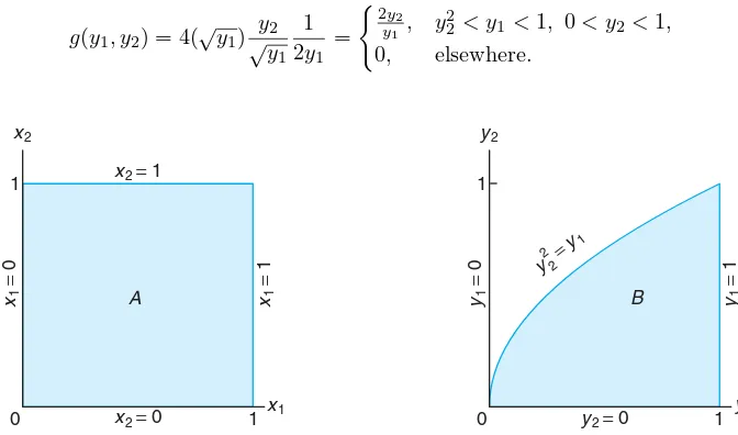
To determine the set B of points in they1y2 plane into which the setA of points in thex1x2 plane is mapped, we write

x1=√y1 and x2=y2/√y1.

Then setting x1 = 0, x2 = 0, x1 = 1, and x2 = 1, the boundaries of set A are transformed to y1 = 0, y2 = 0, y1 = 1, and y2 = √y1, or y22 = y1. The two regions are illustrated in Figure 7.1. Clearly, the transformation is one-to-one, mapping the set A = {(x1, x2) | 0 < x1 < 1, 0 < x2 < 1} into the set B ={(y1, y2)|y22< y1<1, 0< y2<1}. From Theorem 7.4 the joint probability distribution ofY1 andY2 is

g(y1, y2) = 4(√y1) y2

√_y

1 1 2y1

=

_2y 2

y1 , y

2

2 < y1<1, 0< y2<1, 0, elsewhere.

x1

x2

A

0 1

1

x2=0

x2=1

x1

=

0

x1

=

1

y1

y2

B

0 1

1

y2=0

y2 2 ₌y

1

y1

=

0

y1

=

1

Figure 7.1: Mapping setAinto setB.

Problems frequently arise when we wish to find the probability distribution of the random variable Y =u(X) when X is a continuous random variable and the transformation is not one-to-one. That is, to each value xthere corresponds exactly one valuey, but to eachyvalue there corresponds more than onexvalue. For example, suppose that f(x) is positive over the interval −1 < x < 2 and zero elsewhere. Consider the transformation y = x2_{. In this case, x =±}√_{y for} 0< y <1 andx=√y for 1< y <4. For the interval 1< y <4, the probability distribution ofY is found as before, using Theorem 7.3. That is,

g(y) =f[w(y)]|J|= f(

√_y)

2√y , 1< y <4.

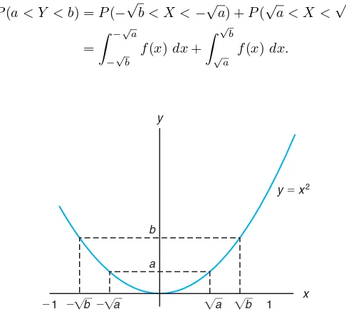
However, when 0< y <1, we may partition the interval−1< x <1 to obtain the two inverse functions

Then to every yvalue there corresponds a singlexvalue for each partition. From Figure 7.2 we see that

P(a < Y < b) =P(−√b < X <−√a) +P(√a < X <√b)

=

−√a

−√b

f(x)dx+

√

b

√_a f(x)dx.

x y

⫺1 1

a b

y ⫽ x2

⫺ b ⫺ a a b

Figure 7.2: Decreasing and increasing function.

Changing the variable of integration from xto y, we obtain

P(a < Y < b) =

a

b

f(−√y)J1 dy+

b

a

f(√y)J2 dy

=−

b

a

f(−√y)J1dy+

b

a

f(√y)J2 dy,

where

J1=

d(−√y)

dy =

−1

2√y =−|J1| and

J2= d(√y)

dy = 1

2√y =|J2|. Hence, we can write

P(a < Y < b) =

b

a

[f(−√y)|J1|+f(√y)|J2|]dy,

and then

g(y) =f(−√y)|J1|+f(√y)|J2|=

f(−√y) +f(√y)

The probability distribution ofY for 0< y <4 may now be written

This procedure for finding g(y) when 0 < y < 1 is generalized in Theorem 7.5 fork inverse functions. For transformations not one-to-one of functions of several variables, the reader is referred toIntroduction to Mathematical Statisticsby Hogg, McKean, and Craig (2005; see the Bibliography).

Theorem 7.5: Suppose that X is a continuous random variable with probability distribution f(x). LetY =u(X) define a transformation between the values ofX andY that is not one-to-one. If the interval over which X is defined can be partitioned into k mutually disjoint sets such that each of the inverse functions

x1=w1(y), x2=w2(y), . . . , xk =wk(y)

ofy=u(x) defines a one-to-one correspondence, then the probability distribution ofY is whenX has a normal distribution with meanµand varianceσ2_.

Solution:LetZ = (X−µ)/σ, where the random variableZ has the standard normal

distri-We shall now find the distribution of the random variable Y =Z2_{. The inverse} solutions of y =z2 _{are z =±}√_{y. If we designatez}

Sinceg(y) is a density function, it follows that

1 = √1 the integral being the area under a gamma probability curve with parameters α= 1/2 andβ = 2. Hence,√π= Γ(1/2) and the density ofY is given by

7.3

Moments and Moment-Generating Functions

In this section, we concentrate on applications of moment-generating functions. The obvious purpose of the moment-generating function is in determining moments of random variables. However, the most important contribution is to establish distributions of functions of random variables.

Ifg(X) =Xr_{forr= 0,1,2,3, . . ., Definition 7.1 yields an expected value called}

the rthmoment about the originof the random variableX, which we denote byµ′

r.

Definition 7.1: _{Therthmoment about the originof the random variableX is given by}

µ′

r=E(Xr) =

⎧

⎨

⎩

x

xr_{f(x), ifXis discrete,}

∞

−∞x

r_{f(x)dx, ifXis continuous.}

Since the first and second moments about the origin are given byµ′

1=E(X) and µ′

2=E(X2), we can write the mean and variance of a random variable as

µ=µ′

1 and σ2=µ′2−µ2.

Although the moments of a random variable can be determined directly from Definition 7.1, an alternative procedure exists. This procedure requires us to utilize a moment-generating function.

Definition 7.2: _{Themoment-generating functionof the random variableXis given byE(e}tX₎

and is denoted byMX(t). Hence,

MX(t) =E(etX) =

⎧

⎨

⎩

x

etxf(x), ifXis discrete,

∞

−∞e

tx_{f(x)dx, ifXis continuous.}

Moment-generating functions will exist only if the sum or integral of Definition 7.2 converges. If a moment-generating function of a random variableX does exist, it can be used to generate all the moments of that variable. The method is described in Theorem 7.6 without proof.

Theorem 7.6: LetX be a random variable with moment-generating functionMX(t). Then

dr_M X(t)

dtr

_t=0

=µ′

r.

Example 7.6: Find the moment-generating function of the binomial random variableX and then use it to verify thatµ=np andσ2_=npq.

Solution:From Definition 7.2 we have MX(t) =

n

x=0 etx

_n

x

pxqn−x₌ n

x=0

_n

x

Recognizing this last sum as the binomial expansion of (pet_+q)n_{, we obtain} which agrees with the results obtained in Chapter 5.

Example 7.7: Show that the moment-generating function of the random variable X having a normal probability distribution with meanµand varianceσ2 _{is given by}

MX(t) = exp

µt+1 2σ

2_t2_.

Solution:From Definition 7.2 the moment-generating function of the normal random variable X is

Completing the square in the exponent, we can write

since the last integral represents the area under a standard normal density curve and hence equals 1.

Although the method of transforming variables provides an effective way of finding the distribution of a function of several variables, there is an alternative and often preferred procedure when the function in question is a linear combination of independent random variables. This procedure utilizes the properties of moment-generating functions discussed in the following four theorems. In keeping with the mathematical scope of this book, we state Theorem 7.7 without proof.

Theorem 7.7: (Uniqueness Theorem)LetX andY be two random variables with

moment-generating functionsMX(t) and MY(t), respectively. IfMX(t) = MY(t) for all

values oft, then X andY have the same probability distribution.

Theorem 7.8: MX+a(t) =eatMX(t).

Proof:MX+a(t) =E[et(X+a)] =eatE(etX) =eatMX(t).

Theorem 7.9: MaX(t) =MX(at).

Proof:MaX(t) =E[et(aX)] =E[e(at)X] =MX(at).

Theorem 7.10: IfX1, X2, . . . , Xnare independent random variables with moment-generating

func-tionsMX1(t), MX2(t), . . . , MXn(t), respectively, andY =X1+X2+· · ·+Xn, then MY(t) =MX1(t)MX2(t)· · ·MXn(t).

The proof of Theorem 7.10 is left for the reader.

Theorems 7.7 through 7.10 are vital for understanding moment-generating func-tions. An example follows to illustrate. There are many situations in which we need to know the distribution of the sum of random variables. We may use Theorems 7.7 and 7.10 and the result of Exercise 7.19 on page 224 to find the distribution of a sum of two independent Poisson random variables with moment-generating functions given by

MX1(t) =e

µ1(e

t

−1) _andM

X2(t) =e

µ2(e

t

−1)_,

respectively. According to Theorem 7.10, the moment-generating function of the random variableY1=X1+X2 is

MY1(t) =MX1(t)MX2(t) =e

µ1(e

t

−1)_eµ2(e

t

−1)_=e(µ1+µ2)(e

t

−1)_,

Linear Combinations of Random Variables

In applied statistics one frequently needs to know the probability distribution of a linear combination of independent normal random variables. Let us obtain the distribution of the random variableY =a1X1+a2X2whenX1is a normal variable with mean µ1 and variance σ21 and X2 is also a normal variable but independent ofX1with meanµ2 and varianceσ22. First, by Theorem 7.10, we find

MY(t) =Ma1X1(t)Ma2X2(t),

and then, using Theorem 7.9, we find

MY(t) =MX1(a1t)MX2(a2t).

Substituting a1t fort and then a2t for t in a moment-generating function of the normal distribution derived in Example 7.7, we have

MY(t) = exp(a1µ1t+a21σ12t2/2 +a2µ2t+a22σ22t2/2) = exp[(a1µ1+a2µ2)t+ (a21σ21+a22σ22)t2/2],

which we recognize as the moment-generating function of a distribution that is normal with meana1µ1+a2µ2 and variancea21σ12+a22σ22.

Generalizing to the case of n independent normal variables, we state the fol-lowing result.

Theorem 7.11: If X1, X2, . . . , Xn are independent random variables having normal distributions

with meansµ1, µ2, . . . , µnand variancesσ12, σ22, . . . , σ2n, respectively, then the

ran-dom variable

Y =a1X1+a2X2+· · ·+anXn

has a normal distribution with mean

µY =a1µ1+a2µ2+· · ·+anµn

and variance

σY2 =a21σ21+a22σ22+· · ·+a2nσ2n.

It is now evident that the Poisson distribution and the normal distribution possess a reproductive property in that the sum of independent random variables having either of these distributions is a random variable that also has the same type of distribution. The chi-squared distribution also has this reproductive property.

Theorem 7.12: If X1, X2, . . . , Xn are mutually independent random variables that have,

respec-tively, chi-squared distributions with v1, v2, . . . , vn degrees of freedom, then the

random variable

Y =X1+X2+· · ·+Xn

has a chi-squared distribution withv=v1+v2+· · ·+vn degrees of freedom.

Proof:By Theorem 7.10 and Exercise 7.21,

MY(t) =MX1(t)MX2(t)· · ·MXn(t) andMXi(t) = (1−2t)

−vi/2

222 Chapter 7 Functions of Random Variables (Optional)

Therefore,

MY(t) = (1−2t)−v1/2(1−2t)−v2/2· · ·(1−2t)−vn/2= (1−2t)−(v1+v2+···+vn)/2,

which we recognize as the moment-generating function of a chi-squared distribution with v=v1+v2+· · ·+vn degrees of freedom.

Corollary 7.1: IfX1, X2, . . . , Xn are independent random variables having identical normal

dis-tributions with meanµand varianceσ2_{, then the random variable}

Y =

has a chi-squared distribution withv=ndegrees of freedom.

This corollary is an immediate consequence of Example 7.5. It establishes a re-lationship between the very important chi-squared distribution and the normal distribution. It also should provide the reader with a clear idea of what we mean by the parameter that we call degrees of freedom. In future chapters, the notion of degrees of freedom will play an increasingly important role.

Corollary 7.2: IfX1, X2, . . . , Xn are independent random variables andXi follows a normal

dis-has a chi-squared distribution withv=ndegrees of freedom.

Exercises

7.1 _{LetX be a random variable with probability}

f(x) = 1

3, x= 1,2,3, 0, elsewhere.

Find the probability distribution of the random vari-ableY = 2X−1.

7.2 _{LetX be a binomial random variable with} prob-ability distribution

Find the probability distribution of the random vari-ableY =X2.

7.3 _{LetX1andX2be discrete random variables with}

the joint multinomial distribution

f(x1, x2) elsewhere. Find the joint probability distribution of

Y1=X1+X2 andY2=X1−X2.

7.4 _{LetX1andX2be discrete random variables with} joint probability distribution

f(x1, x2) = x1x2

18 , x1= 1,2; x2= 1,2,3, 0, elsewhere.

Exercises 223

7.5 _{LetX have the probability distribution}

f(x) =

1, 0< x <1,

0, elsewhere.

Show that the random variableY =−2 lnXhas a chi-squared distribution with 2 degrees of freedom.

7.6 _{Given the random variable X with probability} distribution

f(x) =

2x, 0< x <1,

0, elsewhere,

find the probability distribution ofY = 8X3_.

7.7 _{The speed of a molecule in a uniform gas at} equi-librium is a random variableV whose probability dis-tribution is given by

f(v) =

kv2_e−bv2

, v >0,

0, elsewhere,

where k is an appropriate constant and bdepends on the absolute temperature and mass of the molecule. Find the probability distribution of the kinetic energy of the moleculeW, whereW =mV2/2.

7.8 _{A dealer’s profit, in units of $5000, on a new} au-tomobile is given by Y = X2_{, where X is a random} variable having the density function

f(x) =

2(1−x), 0< x <1,

0, elsewhere.

(a) Find the probability density function of the random variableY.

(b) Using the density function ofY, find the probabil-ity that the profit on the next new automobile sold by this dealership will be less than $500.

7.9 _{The hospital period, in days, for patients} follow-ing treatment for a certain type of kidney disorder is a random variableY =X+ 4, whereX has the density function

f(x) =

₃₂

(x+4)3, x >0,

0, elsewhere.

(a) Find the probability density function of the random variableY.

(b) Using the density function ofY, find the probabil-ity that the hospital period for a patient following this treatment will exceed 8 days.

7.10 _{The random variables X and Y, representing} the weights of creams and toffees, respectively, in 1-kilogram boxes of chocolates containing a mixture of creams, toffees, and cordials, have the joint density function

f(x, y) =

24xy, 0≤x≤1, 0≤y≤1, x+y≤1,

0, elsewhere.

(a) Find the probability density function of the random variableZ=X+Y.

(b) Using the density function ofZ, find the probabil-ity that, in a given box, the sum of the weights of creams and toffees accounts for at least 1/2 but less than 3/4 of the total weight.

7.11 _{The amount of kerosene, in thousands of liters,} in a tank at the beginning of any day is a random amountY from which a random amountX is sold dur-ing that day. Assume that the joint density function of these variables is given by

f(x, y) =

2, 0< x < y, 0< y <1,

0, elsewhere.

Find the probability density function for the amount of kerosene left in the tank at the end of the day.

7.12 _{LetX1andX2be independent random variables} each having the probability distribution

f(x) =

e−x_{, x >0,}

0, elsewhere.

Show that the random variablesY1 and Y2 are inde-pendent whenY1=X1+X2 andY2=X1/(X1+X2).

7.13 _{A current of}I_{amperes flowing through a} resis-tance of R _{ohms varies according to the probability} distribution

f(i) =

6i(1−i), 0< i <1,

0, elsewhere.

If the resistance varies independently of the current ac-cording to the probability distribution

g(r) =

2r, 0< r <1,

0, elsewhere,

find the probability distribution for the powerW =

I2Rwatts.

7.14 _{Let X be a random variable with probability} distribution

f(x) = 1+x

2 , −1< x <1, 0, elsewhere.

7.15 _{LetX have the probability distribution}

f(x) =

_2(x+1)

9 , −1< x <2, 0, elsewhere.

Find the probability distribution of the random vari-ableY =X2_.

7.16 _{Show that the rth moment about the origin of} the gamma distribution is

µ′

and then use the gamma function to evaluate the inte-gral.]

7.17 _{A random variable X has the discrete uniform} distribution

f(x;k) = 1

k, x= 1,2, . . . , k,

0, elsewhere.

Show that the moment-generating function of X is

MX(t) =

et_(1−ekt₎ k(1−et₎ .

7.18 _{A random variable X has the geometric} distri-bution g(x;p) = pqx−1 _{forx= 1,2,3, . . .. Show that} the moment-generating function ofX is

MX(t) = pe t

1−qet, t <lnq,

and then use MX(t) to find the mean and variance of

the geometric distribution.

7.19 _{A random variableX has the Poisson} distribu-tionp(x;µ) =e−µ_µx_{/x! forx= 0,1,2, . . .. Show that}

the moment-generating function ofX is

MX(t) =eµ(e

t

−1)_.

UsingMX(t), find the mean and variance of the

Pois-son distribution.

7.20 _{The moment-generating function of a certain} Poisson random variableX is given by

MX(t) =e4(e

t

−1)_.

FindP(µ−2σ < X < µ+ 2σ).

7.21 _{Show that the moment-generating function of} the random variableX having a chi-squared distribu-tion withvdegrees of freedom is

MX(t) = (1−2t) −v/2_.

7.22 _{Using the moment-generating function of} Exer-cise 7.21, show that the mean and variance of the chi-squared distribution withvdegrees of freedom are, re-spectively,vand 2v.

7.23 _{If bothX andY, distributed independently,} fol-low exponential distributions with mean parameter 1, find the distributions of

(a)U =X+Y; (b)V =X/(X+Y).

7.24 _{By expanding e}tx_{in a Maclaurin series and} in-tegrating term by term, show that