Probability Statistics for Engineers Scientists

(1)

Probability & Statistics for

Engineers & Scientists

N I N T H

E D I T I O N

Ronald E. Walpole

Roanoke College

Raymond H. Myers

Virginia Tech

Sharon L. Myers

Radford University

Keying Ye

University of Texas at San Antonio

(2)

Chapter 11 Simple Linear Regression and

Correlation

11.1 Introduction to Linear Regression

Often, in practice, one is called upon to solve problems involving sets of variables when it is known that there exists some inherent relationship among the variables. For example, in an industrial situation it may be known that the tar content in the outlet stream in a chemical process is related to the inlet temperature. It may be of interest to develop a method of prediction, that is, a procedure for estimating the tar content for various levels of the inlet temperature from experimental infor-mation. Now, of course, it is highly likely that for many example runs in which the inlet temperature is the same, say 130◦_{C, the outlet tar content will not be the}

same. This is much like what happens when we study several automobiles with the same engine volume. They will not all have the same gas mileage. Houses in the same part of the country that have the same square footage of living space will not all be sold for the same price. Tar content, gas mileage (mpg), and the price of houses (in thousands of dollars) are natural dependent variables, or responses, in these three scenarios. Inlet temperature, engine volume (cubic feet), and square feet of living space are, respectively, naturalindependent variables, orregressors. A reasonable form of a relationship between theresponseY and the regressor xis the linear relationship

Y =β0+β1x,

where, of course, β0 is the intercept and β1 is the slope. The relationship is

illustrated in Figure 11.1.

If the relationship is exact, then it is a deterministic relationship between two scientific variables and there is no random or probabilistic component to it. However, in the examples listed above, as well as in countless other scientific and engineering phenomena, the relationship is not deterministic (i.e., a given xdoes not always give the same value for Y). As a result, important problems here are probabilistic in nature since the relationship above cannot be viewed as being exact. The concept ofregression analysisdeals with finding the best relationship

(3)

x Y

}

β0

Y=

0+ β β

1x

Figure 11.1: A linear relationship;β0: intercept;β1: slope.

betweenY andx, quantifying the strength of that relationship, and using methods that allow for prediction of the response values given values of the regressorx.

In many applications, there will be more than one regressor (i.e., more than one independent variable that helps to explain Y). For example, in the case where the response is the price of a house, one would expect the age of the house to contribute to the explanation of the price, so in this case the multiple regression structure might be written

Y =β0+β1x1+β2x2,

where Y is price, x1 is square footage, and x2 is age in years. In the next

chap-ter, we will consider problems with multiple regressors. The resulting analysis is termed multiple regression, while the analysis of the single regressor case is calledsimple regression. As a second illustration of multiple regression, a chem-ical engineer may be concerned with the amount of hydrogen lost from samples of a particular metal when the material is placed in storage. In this case, there may be two inputs, storage timex1in hours and storage temperaturex2in degrees

centigrade. The response would then be hydrogen lossY in parts per million. In this chapter, we deal with the topic of simple linear regression, treating only the case of a single regressor variable in which the relationship betweenyand

xis linear. For the case of more than one regressor variable, the reader is referred to Chapter 12. Denote a random sample of sizenby the set{(xi, yi); i= 1,2, . . . , n}.

If additional samples were taken using exactly the same values of x, we should expect the y values to vary. Hence, the value yi in the ordered pair (xi, yi) is a

value of some random variableYi.

11.2 The Simple Linear Regression (SLR) Model

(4)

11.2 The Simple Linear Regression Model 391

This random component takes into account considerations that are not being mea-sured or, in fact, are not understood by the scientists or engineers. Indeed, in most applications of regression, the linear equation, sayY =β0+β1x, is an

approxima-tion that is a simplificaapproxima-tion of something unknown and much more complicated. For example, in our illustration involving the response Y= tar content and x= inlet temperature,Y =β0+β1xis likely a reasonable approximation that may be

operative within a confined range onx. More often than not, the models that are simplifications of more complicated and unknown structures are linear in nature (i.e., linear in theparametersβ0andβ1or, in the case of the model involving the

price, size, and age of the house, linear in theparametersβ0,β1, andβ2). These

linear structures are simple and empirical in nature and are thus calledempirical models.

An analysis of the relationship between Y and x requires the statement of a

statistical model. A model is often used by a statistician as a representation of anidealthat essentially defines how we perceive that the data were generated by the system in question. The model must include the set{(xi, yi); i= 1,2, . . . , n}

of data involvingnpairs of (x, y) values. One must bear in mind that the valueyi

depends onxivia a linear structure that also has the random component involved.

The basis for the use of a statistical model relates to how the random variable

Y moves with x and the random component. The model also includes what is assumed about the statistical properties of the random component. The statistical model for simple linear regression is given below. The responseY is related to the independent variablexthrough the equation

Simple Linear

Regression Model Y =β0+β1x+ǫ.

In the above,β0 andβ1are unknown intercept and slope parameters, respectively,

and ǫ is a random variable that is assumed to be distributed withE(ǫ) = 0 and Var(ǫ) =σ2_{. The quantity}_σ2_{is often called the error variance or residual variance.}

From the model above, several things become apparent. The quantity Y is a random variable since ǫ is random. The value x of the regressor variable is not random and, in fact, is measured with negligible error. The quantityǫ, often called a random error or random disturbance, has constant variance. This portion of the assumptions is often called thehomogeneous variance assump-tion. The presence of this random error,ǫ, keeps the model from becoming simply a deterministic equation. Now, the fact that E(ǫ) = 0 implies that at a specific

x the y-values are distributed around the true, or population, regression line

y =β0+β1x. If the model is well chosen (i.e., there are no additional important

regressors and the linear approximation is good within the ranges of the data), then positive and negative errors around the true regression are reasonable. We must keep in mind that in practiceβ0andβ1are not known and must be estimated

(5)

scientist or engineer. Rather, the picture merely describes what the assumptions mean! The regression that the user has at his or her disposal will now be described.

x y

ε₁

ε₂ ε₃

ε₄ ε5

“True’’ Regression Line

E

(

Y

)

=β0+β1x

Figure 11.2: Hypothetical (x, y) data scattered around the true regression line for

n= 5.

The Fitted Regression Line

An important aspect of regression analysis is, very simply, to estimate the parame-tersβ0andβ1 (i.e., estimate the so-calledregression coefficients). The method

of estimation will be discussed in the next section. Suppose we denote the esti-mates b0 for β0 and b1 for β1. Then the estimated orﬁtted regression line is

given by

ˆ

y=b0+b1x,

where ˆy is the predicted or fitted value. Obviously, the fitted line is an estimate of the true regression line. We expect that the fitted line should be closer to the true regression line when a large amount of data are available. In the following example, we illustrate the fitted line for a real-life pollution study.

One of the more challenging problems confronting the water pollution control field is presented by the tanning industry. Tannery wastes are chemically complex. They are characterized by high values of chemical oxygen demand, volatile solids, and other pollution measures. Consider the experimental data in Table 11.1, which were obtained from 33 samples of chemically treated waste in a study conducted at Virginia Tech. Readings on x, the percent reduction in total solids, andy, the percent reduction in chemical oxygen demand, were recorded.

(6)

11.2 The Simple Linear Regression Model 393

Table 11.1: Measures of Reduction in Solids and Oxygen Demand

Solids Reduction, Oxygen Demand Solids Reduction, Oxygen Demand

x(%) Reduction,y(%) x(%) Reduction,y(%)

Figure 11.3: Scatter diagram with regression lines.

(7)

Another Look at the Model Assumptions

It may be instructive to revisit the simple linear regression model presented previ-ously and discuss in a graphical sense how it relates to the so-called true regression. Let us expand on Figure 11.2 by illustrating not merely where theǫifall on a graph

but also what the implication is of the normality assumption on theǫi.

Suppose we have a simple linear regression withn= 6 evenly spaced values ofx

and a singley-value at eachx. Consider the graph in Figure 11.4. This illustration should give the reader a clear representation of the model and the assumptions involved. The line in the graph is the true regression line. The points plotted are actual (y, x) points which are scattered about the line. Each point is on its own normal distribution with the center of the distribution (i.e., the mean of y) falling on the line. This is certainly expected sinceE(Y) =β0+β1x. As a result,

the true regression line goes through the means of the response, and the actual observations are on the distribution around the means. Note also that all distributions have the same variance, which we referred to as σ2. Of course, the deviation between an individual y and the point on the line will be its individual

ǫ value. This is clear since

yi−E(Yi) =yi−(β0+β1xi) =ǫi.

Thus, at a givenx,Y and the correspondingǫboth have varianceσ2_.

x Y

µY x= β0

+ β1x /

x1 x2 x3 x4 x5 x6

Figure 11.4: Individual observations around true regression line.

Note also that we have written the true regression line here asμY|x=β0+β1x

in order to reaffirm that the line goes through the mean of theY random variable.

11.3 Least Squares and the Fitted Model

(8)

11.3 Least Squares and the Fitted Model 395

for β1. This of course allows for the computation of predicted values from the

fitted line ˆy = b0+b1x and other types of analyses and diagnostic information

that will ascertain the strength of the relationship and the adequacy of the fitted model. Before we discuss the method of least squares estimation, it is important to introduce the concept of aresidual. A residual is essentially an error in the fit of the model ˆy=b0+b1x.

Residual: Error in Fit

Given a set of regression data {(xi, yi);i= 1,2, . . . , n} and a fitted model, ˆyi =

b0+b1xi, theith residualei is given by

ei=yi−yˆi, i= 1,2, . . . , n.

Obviously, if a set ofnresiduals is large, then the fit of the model is not good. Small residuals are a sign of a good fit. Another interesting relationship which is useful at times is the following:

yi=b0+b1xi+ei.

The use of the above equation should result in clarification of the distinction be-tween the residuals, ei, and the conceptual model errors, ǫi. One must bear in

mind that whereas the ǫi are not observed, theei not only are observed but also

play an important role in the total analysis.

Figure 11.5 depicts the line fit to this set of data, namely ˆy=b0+b1x, and the

line reflecting the modelμY|x=β0+β1x. Now, of course,β0 andβ1are unknown

parameters. The fitted line is an estimate of the line produced by the statistical model. Keep in mind that the line μY|x=β0+β1xis not known.

x

y

µY x β0 β1x

y^=b0+

= +

b1x

|

(

xi, yi

)

}

ei

{

ε_i

Figure 11.5: Comparingǫi with the residual,ei.

The Method of Least Squares

We shall findb0 andb1, the estimates ofβ0andβ1, so that the sum of the squares

(9)

minimization procedure for estimating the parameters is called the method of least squares. Hence, we shall findaandb so as to minimize

SSE=

Differentiating SSE with respect tob0and b1, we have

∂(SSE)

Setting the partial derivatives equal to zero and rearranging the terms, we obtain the equations (called thenormal equations)

nb0+b1

which may be solved simultaneously to yield computing formulas forb0andb1.

Estimating the Regression Coefficients

Given the sample{(xi, yi); i= 1,2, . . . , n}, the least squares estimates b0 andb1

of the regression coefficientsβ0 andβ1 are computed from the formulas

b1=

The calculations of b0 and b1, using the data of Table 11.1, are illustrated by the

following example.

Example 11.1: Estimate the regression line for the pollution data of Table 11.1.

Solution: 33

(33)(41,355)−(1104)(1124)

(33)(41,086)−(1104)2 = 0.903643 and

b0= 1124−(0.903643)(1104)

33 = 3.829633. Thus, the estimated regression line is given by

ˆ

y= 3.8296 + 0.9036x.

(10)

11.3 Least Squares and the Fitted Model 397

31% reduction in the chemical oxygen demand may be interpreted as an estimate of the population mean μY|30 or as an estimate of a new observation when the

reduction in total solids is 30%. Such estimates, however, are subject to error. Even if the experiment were controlled so that the reduction in total solids was 30%, it is unlikely that we would measure a reduction in the chemical oxygen demand exactly equal to 31%. In fact, the original data recorded in Table 11.1 show that measurements of 25% and 35% were recorded for the reduction in oxygen demand when the reduction in total solids was kept at 30%.

What Is Good about Least Squares?

It should be noted that the least squares criterion is designed to provide a fitted line that results in a “closeness” between the line and the plotted points. There are many ways of measuring closeness. For example, one may wish to determineb0

andb1 for which n

i=1|

yi−yˆi|is minimized or for which n

i=1|

yi−yˆi|1.5is minimized.

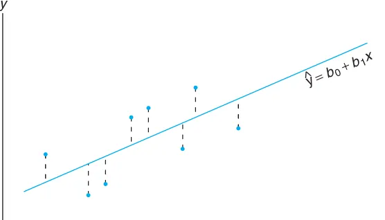
These are both viable and reasonable methods. Note that both of these, as well as the least squares procedure, result in forcing residuals to be “small” in some sense. One should remember that the residuals are the empirical counterpart to the ǫ values. Figure 11.6 illustrates a set of residuals. One should note that the fitted line has predicted values as points on the line and hence the residuals are vertical deviations from points to the line. As a result, the least squares procedure produces a line that minimizes the sum of squares of vertical deviations

from the points to the line.

x y

y

^=b0+

b1x

(11)

398 Chapter 11 Simple Linear Regression and Correlation

Exercises

11.1 A study was conducted at Virginia Tech to de-termine if certain static arm-strength measures have an inﬂuence on the “dynamic lift” characteristics of an individual. Twenty-ﬁve individuals were subjected to strength tests and then were asked to perform a weight-lifting test in which weight was dynamically lifted over-head. The data are given here.

Arm Dynamic

Individual Strength,x Lift, y

1 (a) Estimateβ0 andβ1 for the linear regression curve

μY|x=β0+β1x.

(b) Find a point estimate ofμY|30.

(c) Plot the residuals versus the x’s (arm strength). Comment.

11.2 The grades of a class of 9 students on a midterm report (x) and on the ﬁnal examination (y) are as fol-lows:

x 77 50 71 72 81 94 96 99 67

y 82 66 78 34 47 85 99 99 68 (a) Estimate the linear regression line.

(b) Estimate the ﬁnal examination grade of a student who received a grade of 85 on the midterm report.

11.3 The amounts of a chemical compoundythat dis-solved in 100 grams of water at various temperatures

xwere recorded as follows:

x(◦_C) _y_(grams) (a) Find the equation of the regression line. (b) Graph the line on a scatter diagram.

(c) Estimate the amount of chemical that will dissolve in 100 grams of water at 50◦_C.

11.4 The following data were collected to determine the relationship between pressure and the correspond-ing scale readcorrespond-ing for the purpose of calibration.

Pressure, x(lb/sq in.) Scale Reading, y

10 13

(a) Find the equation of the regression line.

(b) The purpose of calibration in this application is to estimate pressure from an observed scale reading. Estimate the pressure for a scale reading of 54 using ˆ

x= (54−b0)/b1.

11.5 A study was made on the amount of converted sugar in a certain process at various temperatures. The data were coded and recorded as follows:

Temperature, x Converted Sugar,y

1.0 (a) Estimate the linear regression line.

(12)

/ /

Exercises 399

11.6 In a certain type of metal test specimen, the nor-mal stress on a specimen is known to be functionally related to the shear resistance. The following is a set of coded experimental data on the two variables:

Normal Stress,x Shear Resistance,y

26.8 26.5

(b) Estimate the shear resistance for a normal stress of 24.5.

11.7 The following is a portion of a classic data set called the “pilot plot data” in Fitting Equations to Data by Daniel and Wood, published in 1971. The responseyis the acid content of material produced by titration, whereas the regressor x is the organic acid content produced by extraction and weighing.

y x y x

(a) Plot the data; does it appear that a simple linear regression will be a suitable model?

(b) Fit a simple linear regression; estimate a slope and intercept.

(c) Graph the regression line on the plot in (a).

11.8 A mathematics placement test is given to all en-tering freshmen at a small college. A student who re-ceives a grade below 35 is denied admission to the regu-lar mathematics course and placed in a remedial class. The placement test scores and the ﬁnal grades for 20 students who took the regular course were recorded. (a) Plot a scatter diagram.

(b) Find the equation of the regression line to predict course grades from placement test scores.

(c) Graph the line on the scatter diagram.

(d) If 60 is the minimum passing grade, below which placement test score should students in the future be denied admission to this course?

Placement Test Course Grade

50 53

11.9 A study was made by a retail merchant to deter-mine the relation between weekly advertising expendi-tures and sales.

Advertising Costs ($) Sales ($)

40 385

(a) Plot a scatter diagram.

(b) Find the equation of the regression line to predict weekly sales from advertising expenditures. (c) Estimate the weekly sales when advertising costs

are $35.

(d) Plot the residuals versus advertising costs. Com-ment.

11.10 The following data are the selling priceszof a certain make and model of used carwyears old. Fit a curve of the formμz|w=γδw by means of the

nonlin-ear sample regression equation ˆz =cdw. [Hint: Write ln ˆz= lnc+ (lnd)w=b0+b1w.]

w(years) z(dollars) w(years) z(dollars)

1 6350 3 5395

2 5695 5 4985

(13)

11.11 The thrust of an engine (y) is a function of exhaust temperature (x) in ◦F when other important variables are held constant. Consider the following data.

y x y x

4300 1760 4010 1665 4650 1652 3810 1550 3200 1485 4500 1700 3150 1390 3008 1270 4950 1820

(a) Plot the data.

(b) Fit a simple linear regression to the data and plot the line through the data.

11.12 A study was done to study the eﬀect of ambi-ent temperature xon the electric power consumed by a chemical plant y. Other factors were held constant, and the data were collected from an experimental pilot plant.

(a) Plot the data.

(b) Estimate the slope and intercept in a simple linear regression model.

(c) Predict power consumption for an ambient temper-ature of 65◦_F.

11.13 A study of the amount of rainfall and the quan-tity of air pollution removed produced the following

data:

Daily Rainfall, Particulate Removed,

x(0.01 cm) y(µg/m3)

(a) Find the equation of the regression line to predict the particulate removed from the amount of daily rainfall.

(b) Estimate the amount of particulate removed when the daily rainfall isx= 4.8 units.

11.14 A professor in the School of Business in a uni-versity polled a dozen colleagues about the number of professional meetings they attended in the past ﬁve years (x) and the number of papers they submitted to refereed journals (y) during the same period. The summary data are given as follows:

n= 12, x¯= 4, y¯= 12,

Fit a simple linear regression model betweenxandyby ﬁnding out the estimates of intercept and slope. Com-ment on whether attending more professional meetings would result in publishing more papers.

11.4 Properties of the Least Squares Estimators

In addition to the assumptions that the error term in the model

Yi=β0+β1xi+ǫi

is a random variable with mean 0 and constant varianceσ2_{, suppose that we make}

the further assumption that ǫ1, ǫ2, . . . , ǫn are independent from run to run in the

experiment. This provides a foundation for finding the means and variances for the estimators of β0 andβ1.

It is important to remember that our values of b0 and b1, based on a given

sample of nobservations, are only estimates of true parameters β0 andβ1. If the

experiment is repeated over and over again, each time using the same fixed values of x, the resulting estimates ofβ0 and β1 will most likely differ from experiment

to experiment. These different estimates may be viewed as values assumed by the random variablesB0andB1, while b0 andb1 are specific realizations.

Since the values ofxremain fixed, the values ofB0 andB1depend on the

(14)

11.4 Properties of the Least Squares Estimators 401

Mean and Variance of Estimators

In what follows, we show that the estimatorB1is unbiased forβ1and demonstrate

the variances of both B0 and B1. This will begin a series of developments that

lead to hypothesis testing and confidence interval estimation on the intercept and slope.

It can also be shown (Review Exercise 11.60 on page 438) that the random variableB0is normally distributed with

meanμB0 =β0 and varianceσ

From the foregoing results, it is apparent that theleast squares estimators for

β0 and β1 are both unbiased estimators.

Partition of Total Variability and Estimation of

σ

2

To draw inferences on β0 and β1, it becomes necessary to arrive at an estimate

of the parameterσ2 _{appearing in the two preceding variance formulas for}_B 0 and

(15)

experimental error variation around the regression line. In much of what follows, it is advantageous to use the notation

Sxx= n

i=1

(xi−x¯)2, Syy = n

i=1

(yi−y¯)2, Sxy= n

i=1

(xi−x¯)(yi−y¯).

Now we may write the error sum of squares as follows:

SSE=

n

i=1

(yi−b0−b1xi)2= n

i=1

[(yi−y¯)−b1(xi−x¯)]2

=

n

i=1

(yi−y¯)2−2b1 n

i=1

(xi−x¯)(yi−y¯) +b21 n

i=1

(xi−x¯)2

=Syy−2b1Sxy+b12Sxx=Syy−b1Sxy,

the final step following from the fact thatb1=Sxy/Sxx.

Theorem 11.1: An unbiased estimate ofσ2 _is

s2= SSE

n−2 =

n

i=1

(yi−yˆi)2

n−2 =

Syy−b1Sxy

n−2 .

The proof of Theorem 11.1 is left as an exercise (see Review Exercise 11.59).

The Estimator of

σ

2

_{as a Mean Squared Error}

One should observe the result of Theorem 11.1 in order to gain some intuition about the estimator of σ2_{. The parameter} _σ2 _{measures variance or squared deviations}

betweenY values and their mean given byμY|x (i.e., squared deviations between

Y and β0+β1x). Of course, β0+β1x is estimated by ˆy = b0+b1x. Thus, it

would make sense that the variance σ2 _{is best depicted as a squared deviation of}

the typical observationyi from the estimated mean, ˆyi, which is the corresponding

point on the fitted line. Thus, (yi−yˆi)2 values reveal the appropriate variance,

much like the way (yi−y¯)2 values measure variance when one is sampling in a

nonregression scenario. In other words, ¯y estimates the mean in the latter simple situation, whereas ˆyiestimates the mean ofyiin a regression structure. Now, what

about the divisorn−2? In future sections, we shall note that these are the degrees of freedom associated with the estimators2_of_σ2_{. Whereas in the standard normal}

i.i.d. scenario, one degree of freedom is subtracted fromnin the denominator and a reasonable explanation is that one parameter is estimated, namely the meanμby, say, ¯y, but in the regression problem,two parameters are estimated, namely

β0 andβ1 byb0 andb1. Thus, the important parameterσ2, estimated by

s2=

n

i=1

(yi−yˆi)2/(n−2),

(16)

11.5 Inferences Concerning the Regression Coefficients 403

11.5 Inferences Concerning the Regression Coefficients

Aside from merely estimating the linear relationship betweenxandY for purposes of prediction, the experimenter may also be interested in drawing certain inferences about the slope and intercept. In order to allow for the testing of hypotheses and the construction of confidence intervals onβ0andβ1, one must be willing to make

the further assumption that eachǫi, i= 1,2, . . . , n, is normally distributed. This

assumption implies that Y1, Y2, . . . , Yn are also normally distributed, each with

probability distributionn(yi;β0+β1xi, σ).

From Section 11.4 we know thatB1follows a normal distribution. It turns out

that under the normality assumption, a result very much analogous to that given in Theorem 8.4 allows us to conclude that (n−2)S2_/σ2 _{is a chi-squared variable}

with n−2 degrees of freedom, independent of the random variable B1. Theorem

8.5 then assures us that the statistic

T = (B1−β1)/(σ/

√

Sxx)

S/σ =

B1−β1

S/√Sxx

has at-distribution withn−2 degrees of freedom. The statisticT can be used to construct a 100(1−α)% confidence interval for the coefficientβ1.

Confidence Interval forβ1

A 100(1−α)% confidence interval for the parameter β1 in the regression line

μY|x=β0+β1xis

b1−tα/2

s

√

Sxx

< β1< b1+tα/2

s

√

Sxx

,

wheretα/2 is a value of thet-distribution withn−2 degrees of freedom.

Example 11.2: Find a 95% confidence interval forβ1in the regression lineμY|x=β0+β1x, based

on the pollution data of Table 11.1.

Solution: From the results given in Example 11.1 we find that Sxx = 4152.18 and Sxy =

3752.09. In addition, we find that Syy = 3713.88. Recall that b1 = 0.903643.

Hence,

s2= Syy−b1Sxy

n−2 =

3713.88−(0.903643)(3752.09)

31 = 10.4299.

Therefore, taking the square root, we obtains= 3.2295. Using Table A.4, we find

t0.025 ≈2.045 for 31 degrees of freedom. Therefore, a 95% confidence interval for

β1is

0.903643−(2.045)(3√ .2295)

4152.18 < β <0.903643 +

(2.045)(3.2295)

√

4152.18 ,

which simplifies to

(17)

Hypothesis Testing on the Slope

To test the null hypothesis H0 that β1 = β10 against a suitable alternative, we

again use the t-distribution with n−2 degrees of freedom to establish a critical region and then base our decision on the value of

t=b1−β10

s/√Sxx

.

The method is illustrated by the following example.

Example 11.3: Using the estimated valueb1= 0.903643 of Example 11.1, test the hypothesis that

β1= 1.0 against the alternative thatβ1<1.0.

Solution:The hypotheses areH0: β1= 1.0 andH1: β1<1.0. So

t= 0.903643−1.0

3.2295/√4152.18 =−1.92,

with n−2 = 31 degrees of freedom (P ≈0.03).

Decision: Thet-value is significant at the 0.03 level, suggesting strong evidence that β1<1.0.

One importantt-test on the slope is the test of the hypothesis

H0: β1= 0 versus H1: β1= 0.

When the null hypothesis is not rejected, the conclusion is that there is no signifi-cant linear relationship betweenE(y) and the independent variablex. The plot of the data for Example 11.1 would suggest that a linear relationship exists. However, in some applications in whichσ2_{is large and thus considerable “noise” is present in}

the data, a plot, while useful, may not produce clear information for the researcher. Rejection of H0 above implies that a significant linear regression exists.

Figure 11.7 displays aMINITABprintout showing thet-test for

H0: β1= 0 versus H1: β1= 0,

for the data of Example 11.1. Note the regression coefficient (Coef), standard error (SE Coef), t-value (T), andP-value (P). The null hypothesis is rejected. Clearly, there is a significant linear relationship between mean chemical oxygen demand reduction and solids reduction. Note that thet-statistic is computed as

t= coefficient standard error =

b1

s/√Sxx

.

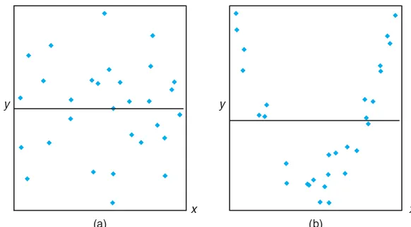
The failure to reject H0: β1 = 0 suggests that there is no linear relationship

between Y and x. Figure 11.8 is an illustration of the implication of this result. It may mean that changing x has little impact on changes inY, as seen in (a). However, it may also indicate that the true relationship is nonlinear, as indicated by (b).

WhenH0:β1= 0 is rejected, there is an implication that the linear term in x

(18)

Regression Analysis: COD versus Per_Red

The regression equation is COD = 3.83 + 0.904 Per_Red

Predictor Coef SE Coef T P

Constant 3.830 1.768 2.17 0.038 Per_Red 0.90364 0.05012 18.03 0.000

S = 3.22954 R-Sq = 91.3% R-Sq(adj) = 91.0% Analysis of Variance

Source DF SS MS F P

Regression 1 3390.6 3390.6 325.08 0.000 Residual Error 31 323.3 10.4

Total 32 3713.9

Figure 11.7: MINITABprintout for t-test for data of Example 11.1.

x

(a)

y

x

(b)

y

Figure 11.8: The hypothesisH0:β1= 0 is not rejected.

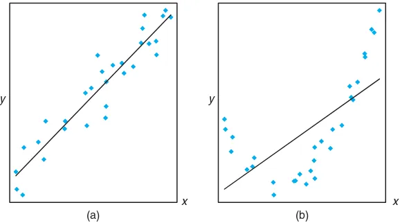
plots in Figure 11.9 illustrate possible scenarios. As depicted in (a) of the figure, rejection ofH0 may suggest that the relationship is, indeed, linear. As indicated

in (b), it may suggest that while the model does contain a linear effect, a better representation may be found by including a polynomial (perhaps quadratic) term (i.e., terms that supplement the linear term).

Statistical Inference on the Intercept

Confidence intervals and hypothesis testing on the coefficientβ0may be established

from the fact thatB0 is also normally distributed. It is not difficult to show that

T = B0−β0

S

%

n

i=1

x2

(19)

x

(a)

y

x

(b)

y

Figure 11.9: The hypothesisH0:β1= 0 is rejected.

has at-distribution withn−2 degrees of freedom from which we may construct a 100(1−α)% confidence interval forα.

Confidence Interval forβ0

A 100(1−α)% confidence interval for the parameter β0 in the regression line

μY|x=β0+β1xis

b0−tα/2

s

√

nSxx

( ) ) *

n

i=1

x2

i < β0< b0+tα/2

s

√

nSxx

( ) ) *

n

i=1

x2 i,

Example 11.4: Find a 95% confidence interval forβ0 in the regression lineμY|x=β0+β1x, based

on the data of Table 11.1.

Solution:In Examples 11.1 and 11.2, we found that

Sxx= 4152.18 and s= 3.2295.

From Example 11.1 we had

n

i=1

x2i = 41,086 and b0= 3.829633.

Using Table A.4, we find t0.025 ≈ 2.045 for 31 degrees of freedom. Therefore, a

95% confidence interval for β0 is

3.829633−(2.045)(3.2295) √

41,086

(33)(4152.18) < β0<3.829633 +

(2.045)(3.2295)√41,086

(33)(4152.18) ,

(20)

To test the null hypothesis H0 that β0 = β00 against a suitable alternative,

we can use thet-distribution withn−2 degrees of freedom to establish a critical region and then base our decision on the value of

t= b0−β00

s

%

n

i=1

x2

i/(nSxx)

.

Example 11.5: Using the estimated valueb0= 3.829633 of Example 11.1, test the hypothesis that

β0= 0 at the 0.05 level of significance against the alternative that β0= 0. Solution:The hypotheses areH0: β0= 0 andH1: β0= 0. So

t= 3.829633−0

3.229541,086/[(33)(4152.18)] = 2.17,

with 31 degrees of freedom. Thus, P = P-value ≈ 0.038 and we conclude that

β0= 0. Note that this is merely Coef/StDev, as we see in theMINITABprintout

in Figure 11.7. The SE Coef is the standard error of the estimated intercept.

A Measure of Quality of Fit: Coefficient of Determination

Note in Figure 11.7 that an item denoted by R-Sq is given with a value of 91.3%. This quantity, R2_{, is called the} _{coefficient of determination}_{. This quantity is}

a measure of the proportion of variability explained by the ﬁtted model. In Section 11.8, we shall introduce the notion of an analysis-of-variance approach to hypothesis testing in regression. The analysis-of-variance approach makes use

of the error sum of squaresSSE=

n

i=1

(yi−yˆi)2and thetotal corrected sum of

squares SST =

n

i=1

(yi−y¯i)2. The latter represents the variation in the response

values thatideallywould be explained by the model. TheSSEvalue is the variation due to error, or variation unexplained. Clearly, if SSE = 0, all variation is explained. The quantity that represents variation explained isSST −SSE. The

R2_is

Coeff. of determination: R2_{= 1}₋SSE

SST.

Note that if the fit is perfect,all residuals are zero, and thusR2_{= 1}_._{0. But if}_SSE

is only slightly smaller thanSST,R2_≈_{0. Note from the printout in Figure 11.7}

that the coefficient of determination suggests that the model fit to the data explains 91.3% of the variability observed in the response, the reduction in chemical oxygen demand.

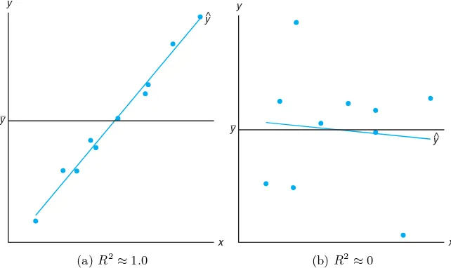
Figure 11.10 provides an illustration of a good fit (R2_≈₁_._{0) in plot (a) and a}

poor fit (R2_≈_{0) in plot (b).}

Pitfalls in the Use of

R

2

Analysts quote values of R2 _{quite often, perhaps due to its simplicity. However,}

(21)

x y

y

y^

(a)R2

≈1.0

x y

y

y^

(b)R2

≈0

Figure 11.10: Plots depicting a very good fit and a poor fit.

size of the regression data set and the type of application. Clearly, 0 ≤R2 _≤ ₁

and the upper bound is achieved when the fit to the data is perfect (i.e., all of the residuals are zero). What is an acceptable value for R2_{? This is a difficult}

question to answer. A chemist, charged with doing a linear calibration of a high-precision piece of equipment, certainly expects to experience a very highR2_-value

(perhaps exceeding 0.99), while a behavioral scientist, dealing in data impacted by variability in human behavior, may feel fortunate to experience an R2 as large as 0.70. An experienced model fitter senses when a value is large enough, given the situation confronted. Clearly, some scientific phenomena lend themselves to modeling with more precision than others.

The R2 _{criterion is dangerous to use for comparing}_{competing models} _{for the}

same data set. Adding additional terms to the model (e.g., an additional regressor) decreasesSSEand thus increasesR2_{(or at least does not decrease it). This implies}

thatR2_{can be made artificially high by an unwise practice of}_overﬁtting_{(i.e., the}

inclusion of too many model terms). Thus, the inevitable increase in R2 _enjoyed

by adding an additional term does not imply the additional term was needed. In fact, the simple model may be superior for predicting response values. The role of overfitting and its influence on prediction capability will be discussed at length in Chapter 12 as we visit the notion of models involving more than a single regressor. Suffice it to say at this point that oneshould not subscribe to a model selection process that solely involves the consideration ofR2_.

11.6 Prediction

(22)

11.6 Prediction 409

section, the focus is on errors associated with prediction.

The equation ˆy = b0 +b1x may be used to predict or estimate the mean responseμY|x0 atx=x0, wherex0is not necessarily one of the prechosen values,

or it may be used to predict a single valuey0of the variable Y0, whenx=x0. We

would expect the error of prediction to be higher in the case of a single predicted value than in the case where a mean is predicted. This, then, will affect the width of our intervals for the values being predicted.

Suppose that the experimenter wishes to construct a confidence interval for

μY|x0. We shall use the point estimator ˆY0 = B0+B1x0 to estimate μY|x0 =

β0+β1x. It can be shown that the sampling distribution of ˆY0 is normal with

mean

μY|x0 =E( ˆY0) =E(B0+B1x0) =β0+β1x0=μY|x0

and variance

σ2_Yˆ0=σ

2

B0+B1x0 =σ

2 ¯

Y+B1(x0−¯x)=σ

2

₁

n+

(x0−x¯)2

Sxx

,

the latter following from the fact that Cov( ¯Y , B1) = 0 (see Review Exercise 11.61

on page 438). Thus, a 100(1−α)% confidence interval on the mean responseμY|x0

can now be constructed from the statistic

T = Yˆ0−μY|x0

S1/n+ (x0−x¯)2/Sxx

,

which has at-distribution withn−2 degrees of freedom.

Confidence Interval forμY_|x0

A 100(1−α)% confidence interval for the mean response μY|x0 is

ˆ

y0−tα/2s

%

1

n+

(x0−x¯)2

Sxx

< μY|x0 <yˆ0+tα/2s %

1

n+

(x0−x¯)2

Sxx

,

Example 11.6: Using the data of Table 11.1, construct 95% confidence limits for the mean response

μY|x0.

Solution:From the regression equation we find forx0= 20% solids reduction, say,

ˆ

y0= 3.829633 + (0.903643)(20) = 21.9025.

In addition, ¯x = 33.4545, Sxx = 4152.18, s = 3.2295, and t0.025 ≈ 2.045 for 31

degrees of freedom. Therefore, a 95% confidence interval forμY|20 is

21.9025−(2.045)(3.2295)

"

1 33+

(20−33.4545)2

4152.18 < μY|20

<21.9025 + (2.045)(3.2295)

"

1 33+

(20−33.4545)2

(23)

or simply 20.1071< μY|20<23.6979.

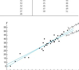
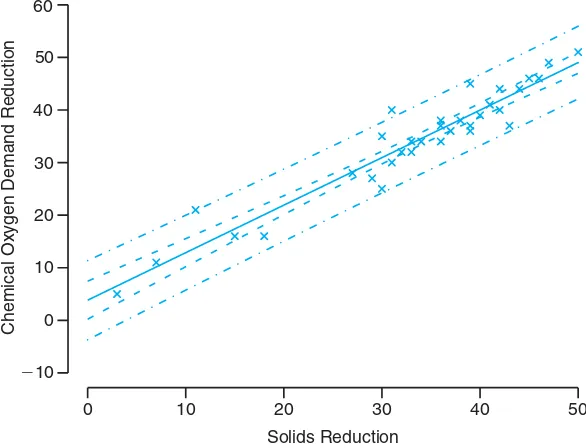
Repeating the previous calculations for each of several different values of x0,

one can obtain the corresponding confidence limits on each μY|x0. Figure 11.11

displays the data points, the estimated regression line, and the upper and lower confidence limits on the mean of Y|x.

x y

0 3 6 9 12 15 18 21 24 27 30 33 36 39 42 45 48 51 54 5

10 15 20 25 30 35 40 45

50 y^=b0+b1x

Figure 11.11: Confidence limits for the mean value ofY|x.

In Example 11.6, we are 95% confident that the population mean reduction in chemical oxygen demand is between 20.1071% and 23.6979% when solid reduction is 20%.

Prediction Interval

Another type of interval that is often misinterpreted and confused with that given forμY|xis the prediction interval for a future observed response. Actually in many

instances, the prediction interval is more relevant to the scientist or engineer than the confidence interval on the mean. In the tar content and inlet temperature ex-ample cited in Section 11.1, there would certainly be interest not only in estimating the mean tar content at a specific temperature but also in constructing an interval that reflects the error in predicting a future observed amount of tar content at the given temperature.

To obtain aprediction intervalfor any single valuey0 of the variableY0, it

is necessary to estimate the variance of the differences between the ordinates ˆy0,

obtained from the computed regression lines in repeated sampling when x= x0,

and the corresponding true ordinatey0. We can think of the difference ˆy0−y0 as

a value of the random variable ˆY0−Y0, whose sampling distribution can be shown

to be normal with mean

μ_Yˆ0−Y0=E( ˆY0−Y0) =E[B0+B1x0−(β0+β1x0+ǫ0)] = 0

and variance

σ2Yˆ0−Y0 =σ

2

B0+B1x0−ǫ0 =σ

2 ¯

Y+B1(x0−x¯)−ǫ0 =σ

2_{1 +} 1

n+

(x0−x¯)2

Sxx

(24)

/ /

Exercises 411

Thus, a 100(1−α)% prediction interval for a single predicted value y0 can be

constructed from the statistic

T = Yˆ0−Y0

S1 + 1/n+ (x0−x¯)2/Sxx

,

which has at-distribution withn−2 degrees of freedom.

Prediction Interval fory0

A 100(1−α)% prediction interval for a single response y0 is given by

ˆ

y0−tα/2s

%

1 + 1

n+

(x0−x¯)2

Sxx

< y0<yˆ0+tα/2s

%

1 + 1

n+

(x0−x¯)2

Sxx

,

Clearly, there is a distinction between the concept of a confidence interval and the prediction interval described previously. The interpretation of the confidence interval is identical to that described for all confidence intervals on population pa-rameters discussed throughout the book. Indeed,μY|x0 is a population parameter.

The computed prediction interval, however, represents an interval that has a prob-ability equal to 1−αof containing not a parameter but a future value y0 of the

random variableY0.

Example 11.7: Using the data of Table 11.1, construct a 95% prediction interval for y0 when

x0= 20%.

Solution:We haven= 33,x0= 20, ¯x= 33.4545, ˆy0 = 21.9025,Sxx= 4152.18,s= 3.2295,

andt0.025≈2.045 for 31 degrees of freedom. Therefore, a 95% prediction interval

fory0 is

21.9025−(2.045)(3.2295)

"

1 + 1 33+

(20−33.4545)2

4152.18 < y0

<21.9025 + (2.045)(3.2295)

"

1 + 1 33+

(20−33.4545)2

4152.18 ,

which simplifies to 15.0585< y0<28.7464.

Figure 11.12 shows another plot of the chemical oxygen demand reduction data, with both the confidence interval on the mean response and the prediction interval on an individual response plotted. The plot reflects a much tighter interval around the regression line in the case of the mean response.

Exercises

11.15 With reference to Exercise 11.1 on page 398, (a) evaluates2

;

(b) test the hypothesis thatβ1 = 0 against the

alter-native thatβ1= 0 at the 0.05 level of signiﬁcance

and interpret the resulting decision.

;

(b) construct a 95% conﬁdence interval forβ0;

(25)

0 10 20 30 40 50

⫺10 0 10 20 30 40 50 60

Solids Reduction

Chemical Oxygen Demand Reduction

Figure 11.12: Confidence and prediction intervals for the chemical oxygen demand reduction data; inside bands indicate the confidence limits for the mean responses and outside bands indicate the prediction limits for the future responses.

;

(c) construct a 95% conﬁdence interval forβ1.

;

11.20 Test the hypothesis that β0 = 10 in Exercise

11.8 on page 399 against the alternative that β0<10. Use a 0.05 level of signiﬁcance.

11.21 Test the hypothesis that β1 = 6 in Exercise 11.9 on page 399 against the alternative thatβ1 <6.

Use a 0.025 level of signiﬁcance.

11.22 Using the value of s2

found in Exercise 11.16(a), construct a 95% conﬁdence interval forμY|85

in Exercise 11.2 on page 398.

11.23 With reference to Exercise 11.6 on page 399, use the value ofs2

found in Exercise 11.18(a) to com-pute

(a) a 95% conﬁdence interval for the mean shear resis-tance whenx= 24.5;

(b) a 95% prediction interval for a single predicted value of the shear resistance whenx= 24.5.

found in Exercise 11.17(a), graph the regression line and the 95% con-ﬁdence bands for the mean responseμY|xfor the data

of Exercise 11.5 on page 398.

found in Exercise 11.17(a), construct a 95% conﬁdence interval for the amount of converted sugar corresponding tox= 1.6 in Exercise 11.5 on page 398.

11.26 With reference to Exercise 11.3 on page 398, use the value ofs2

found in Exercise 11.19(a) to com-pute

(26)

Exercises 413

of chemical that will dissolve in 100 grams of water at 50◦C;

(b) a 99% prediction interval for the amount of chemi-cal that will dissolve in 100 grams of water at 50◦_C.

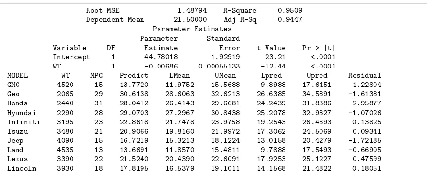
11.27 Consider the regression of mileage for certain automobiles, measured in miles per gallon (mpg) on their weight in pounds (wt). The data are from Con-sumer Reports (April 1997). Part of theSAS output from the procedure is shown in Figure 11.13.

(a) Estimate the mileage for a vehicle weighing 4000 pounds.

(b) Suppose that Honda engineers claim that, on aver-age, the Civic (or any other model weighing 2440 pounds) gets more than 30 mpg. Based on the re-sults of the regression analysis, would you believe that claim? Why or why not?

(c) The design engineers for the Lexus ES300 targeted 18 mpg as being ideal for this model (or any other model weighing 3390 pounds), although it is ex-pected that some variation will be experienced. Is it likely that this target value is realistic? Discuss.

11.28 There are important applications in which, due to known scientiﬁc constraints, the regression line must go through the origin(i.e., the intercept must be zero). In other words, the model should read

Yi=β1xi+ǫi, i= 1,2, . . . , n,

and only a simple parameter requires estimation. The model is often called the regression through the origin model.

(a) Show that the least squares estimator of the slope is

(c) Show that b1 in part (a) is an unbiased estimator

forβ1. That is, showE(B1) =β1.

11.29 Use the data set

y x (a) Plot the data.

(b) Fit a regression line through the origin.

(c) Plot the regression line on the graph with the data. (d) Give a general formula (in terms of theyi and the

slopeb1) for the estimator ofσ2

.

(e) Give a formula for Var(ˆyi),i= 1,2, . . . , n, for this

case.

(f) Plot 95% conﬁdence limits for the mean response on the graph around the regression line.

11.30 For the data in Exercise 11.29, ﬁnd a 95% pre-diction interval atx= 25.

Root MSE 1.48794 R-Square 0.9509

Dependent Mean 21.50000 Adj R-Sq 0.9447 Parameter Estimates

Parameter Standard

Variable DF Estimate Error t Value Pr > |t| Intercept 1 44.78018 1.92919 23.21 <.0001

WT 1 -0.00686 0.00055133 -12.44 <.0001

MODEL WT MPG Predict LMean UMean Lpred Upred Residual

GMC 4520 15 13.7720 11.9752 15.5688 9.8988 17.6451 1.22804 Geo 2065 29 30.6138 28.6063 32.6213 26.6385 34.5891 -1.61381 Honda 2440 31 28.0412 26.4143 29.6681 24.2439 31.8386 2.95877 Hyundai 2290 28 29.0703 27.2967 30.8438 25.2078 32.9327 -1.07026 Infiniti 3195 23 22.8618 21.7478 23.9758 19.2543 26.4693 0.13825 Isuzu 3480 21 20.9066 19.8160 21.9972 17.3062 24.5069 0.09341 Jeep 4090 15 16.7219 15.3213 18.1224 13.0158 20.4279 -1.72185 Land 4535 13 13.6691 11.8570 15.4811 9.7888 17.5493 -0.66905 Lexus 3390 22 21.5240 20.4390 22.6091 17.9253 25.1227 0.47599 Lincoln 3930 18 17.8195 16.5379 19.1011 14.1568 21.4822 0.18051

(27)

11.7 Choice of a Regression Model

Much of what has been presented thus far on regression involving a single inde-pendent variable depends on the assumption that the model chosen is correct, the presumption that μY|x is related to xlinearly in the parameters. Certainly, one

cannot expect the prediction of the response to be good if there are several inde-pendent variables, not considered in the model, that are affecting the response and are varying in the system. In addition, the prediction will certainly be inadequate if the true structure relating μY|x to xis extremely nonlinear in the range of the

variables considered.

Often the simple linear regression model is used even though it is known that the model is something other than linear or that the true structure is unknown. This approach is often sound, particularly when the range ofxis narrow. Thus, the model used becomes an approximating function that one hopes is an adequate rep-resentation of the true picture in the region of interest. One should note, however, the effect of an inadequate model on the results presented thus far. For example, if the true model, unknown to the experimenter, is linear in more than onex, say

μY|x1,x2 =β0+β1x1+β2x2,

then the ordinary least squares estimate b1 = Sxy/Sxx, calculated by only

con-sidering x1 in the experiment, is, under general circumstances, a biased estimate

of the coefficientβ1, the bias being a function of the additional coefficientβ2 (see

Review Exercise 11.65 on page 438). Also, the estimate s2 _for_σ2_{is biased due to}

the additional variable.

11.8 Analysis-of-Variance Approach

Often the problem of analyzing the quality of the estimated regression line is han-dled by an analysis-of-variance (ANOVA) approach: a procedure whereby the total variation in the dependent variable is subdivided into meaningful compo-nents that are then observed and treated in a systematic fashion. The analysis of variance, discussed in Chapter 13, is a powerful resource that is used for many applications.

Suppose that we havenexperimental data points in the usual form (xi, yi) and

that the regression line is estimated. In our estimation of σ2 _{in Section 11.4, we}

established the identity

Syy =b1Sxy+SSE.

An alternative and perhaps more informative formulation is

n

i=1

(yi−y¯)2= n

i=1

(ˆyi−y¯)2+ n

i=1

(yi−yˆi)2.

We have achieved a partitioning of the total corrected sum of squares of y

into two components that should reflect particular meaning to the experimenter. We shall indicate this partitioning symbolically as

(28)

11.8 Analysis-of-Variance Approach 415

The first component on the right,SSR, is called theregression sum of squares, and it reflects the amount of variation in they-values explained by the model, in this case the postulated straight line. The second component is the familiar error sum of squares, which reflects variation about the regression line.

Suppose that we are interested in testing the hypothesis

H0: β1= 0 versusH1: β1= 0,

where the null hypothesis says essentially that the model isμY|x=β0.That is, the

variation inY results from chance or random fluctuations which are independent of the values ofx. This condition is reflected in Figure 11.10(b). Under the conditions of this null hypothesis, it can be shown that SSR/σ2 _and _SSE/σ2 _{are values of}

independent chi-squared variables with 1 andn−2 degrees of freedom, respectively, and then by Theorem 7.12 it follows thatSST /σ2 _{is also a value of a chi-squared}

variable withn−1 degrees of freedom. To test the hypothesis above, we compute

f = SSR/1

SSE/(n−2) =

SSR s2

and rejectH0 at theα-level of significance whenf > fα(1, n−2).

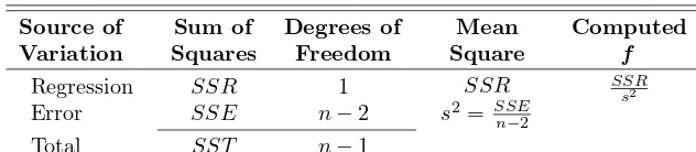
The computations are usually summarized by means of ananalysis-of-variance table, as in Table 11.2. It is customary to refer to the various sums of squares divided by their respective degrees of freedom as themean squares.

Table 11.2: Analysis of Variance for Testingβ1= 0

Source of Sum of Degrees of Mean Computed

Variation Squares Freedom Square f

Regression Error

SSR SSE

1

n−2

SSR s2₌ SSE

n−2

SSR s2

Total SST n−1

When the null hypothesis is rejected, that is, when the computed F-statistic exceeds the critical value fα(1, n−2), we conclude thatthere is a signiﬁcant amount of variation in the response accounted for by the postulated model, the straight-line function. If the F-statistic is in the fail to reject region, we conclude that the data did not reflect sufficient evidence to support the model postulated.

In Section 11.5, a procedure was given whereby the statistic

T =B1−β10

S/√Sxx

is used to test the hypothesis

H0: β1=β10versusH1: β1=β10,

(29)

in the special case in which we are testing

H0: β1= 0 versus H1: β1= 0,

the value of ourT-statistic becomes

t= b1

s/√Sxx

,

and the hypothesis under consideration is identical to that being tested in Table 11.2. Namely, the null hypothesis states that the variation in the response is due merely to chance. The analysis of variance uses the F-distribution rather than thet-distribution. For the two-sided alternative, the two approaches are identical. This we can see by writing

t2=b

2 1Sxx

s2 =

b1Sxy

s2 =

SSR s2 ,

which is identical to thef-value used in the analysis of variance. The basic relation-ship between the t-distribution withv degrees of freedom and theF-distribution with 1 andv degrees of freedom is

t2=f(1, v).

Of course, the t-test allows for testing against a one-sided alternative while the

F-test is restricted to testing against a two-sided alternative.

Annotated Computer Printout for Simple Linear Regression

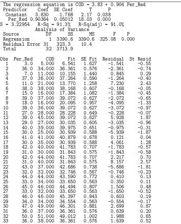
Consider again the chemical oxygen demand reduction data of Table 11.1. Figures 11.14 and 11.15 show more complete annotated computer printouts. Again we illustrate it with MINITAB software. Thet-ratio column indicates tests for null hypotheses of zero values on the parameter. The term “Fit” denotes ˆy-values, often calledﬁtted values. The term “SE Fit” is used in computing confidence intervals on mean response. The itemR2_{is computed as (}_SSR/SST₎_×_{100 and signifies the}

proportion of variation iny explained by the straight-line regression. Also shown are confidence intervals on the mean response and prediction intervals on a new observation.

11.9 Test for Linearity of Regression: Data with Repeated

Observations

In certain kinds of experimental situations, the researcher has the capability of obtaining repeated observations on the response for each value ofx. Although it is not necessary to have these repetitions in order to estimateβ0andβ1, nevertheless

(30)

11.9 Test for Linearity of Regression: Data with Repeated Observations 417

The regression equation is COD = 3.83 + 0.904 Per_Red

Predictor Coef SE Coef T P

Constant 3.830 1.768 2.17 0.038 Per_Red 0.90364 0.05012 18.03 0.000 S = 3.22954 R-Sq = 91.3% R-Sq(adj) = 91.0%

Analysis of Variance

Source DF SS MS F P

Regression 1 3390.6 3390.6 325.08 0.000 Residual Error 31 323.3 10.4

Total 32 3713.9

Obs Per_Red COD Fit SE Fit Residual St Resid

1 3.0 5.000 6.541 1.627 -1.541 -0.55

2 36.0 34.000 36.361 0.576 -2.361 -0.74

3 7.0 11.000 10.155 1.440 0.845 0.29

4 37.0 36.000 37.264 0.590 -1.264 -0.40

5 11.0 21.000 13.770 1.258 7.230 2.43

6 38.0 38.000 38.168 0.607 -0.168 -0.05 7 15.0 16.000 17.384 1.082 -1.384 -0.45 8 39.0 37.000 39.072 0.627 -2.072 -0.65 9 18.0 16.000 20.095 0.957 -4.095 -1.33 10 39.0 36.000 39.072 0.627 -3.072 -0.97 11 27.0 28.000 28.228 0.649 -0.228 -0.07

12 39.0 45.000 39.072 0.627 5.928 1.87

13 29.0 27.000 30.035 0.605 -3.035 -0.96 14 40.0 39.000 39.975 0.651 -0.975 -0.31 15 30.0 25.000 30.939 0.588 -5.939 -1.87

16 41.0 41.000 40.879 0.678 0.121 0.04

17 30.0 35.000 30.939 0.588 4.061 1.28

18 42.0 40.000 41.783 0.707 -1.783 -0.57 19 31.0 30.000 31.843 0.575 -1.843 -0.58

20 42.0 44.000 41.783 0.707 2.217 0.70

21 31.0 40.000 31.843 0.575 8.157 2.57

22 43.0 37.000 42.686 0.738 -5.686 -1.81 23 32.0 32.000 32.746 0.567 -0.746 -0.23

24 44.0 44.000 43.590 0.772 0.410 0.13

25 33.0 34.000 33.650 0.563 0.350 0.11

26 45.0 46.000 44.494 0.807 1.506 0.48

27 33.0 32.000 33.650 0.563 -1.650 -0.52

28 46.0 46.000 45.397 0.843 0.603 0.19

29 34.0 34.000 34.554 0.563 -0.554 -0.17

30 47.0 49.000 46.301 0.881 2.699 0.87

31 36.0 37.000 36.361 0.576 0.639 0.20

32 50.0 51.000 49.012 1.002 1.988 0.65

33 36.0 38.000 36.361 0.576 1.639 0.52

Figure 11.14: MINITABprintout of simple linear regression for chemical oxygen demand reduction data; part I.

Let us select a random sample ofn observations using k distinct values of x, sayx1, x2, . . . , xn, such that the sample containsn1 observed values of the random

variableY1corresponding tox1,n2 observed values ofY2corresponding tox2, . . .,

nk observed values ofYk corresponding toxk. Of necessity,n= k

i=1

(31)

Obs Fit SE Fit 95% CI 95% PI 1 6.541 1.627 ( 3.223, 9.858) (-0.834, 13.916) 2 36.361 0.576 (35.185, 37.537) (29.670, 43.052) 3 10.155 1.440 ( 7.218, 13.092) ( 2.943, 17.367) 4 37.264 0.590 (36.062, 38.467) (30.569, 43.960) 5 13.770 1.258 (11.204, 16.335) ( 6.701, 20.838) 6 38.168 0.607 (36.931, 39.405) (31.466, 44.870) 7 17.384 1.082 (15.177, 19.592) (10.438, 24.331) 8 39.072 0.627 (37.793, 40.351) (32.362, 45.781) 9 20.095 0.957 (18.143, 22.047) (13.225, 26.965) 10 39.072 0.627 (37.793, 40.351) (32.362, 45.781) 11 28.228 0.649 (26.905, 29.551) (21.510, 34.946) 12 39.072 0.627 (37.793, 40.351) (32.362, 45.781) 13 30.035 0.605 (28.802, 31.269) (23.334, 36.737) 14 39.975 0.651 (38.648, 41.303) (33.256, 46.694) 15 30.939 0.588 (29.739, 32.139) (24.244, 37.634) 16 40.879 0.678 (39.497, 42.261) (34.149, 47.609) 17 30.939 0.588 (29.739, 32.139) (24.244, 37.634) 18 41.783 0.707 (40.341, 43.224) (35.040, 48.525) 19 31.843 0.575 (30.669, 33.016) (25.152, 38.533) 20 41.783 0.707 (40.341, 43.224) (35.040, 48.525) 21 31.843 0.575 (30.669, 33.016) (25.152, 38.533) 22 42.686 0.738 (41.181, 44.192) (35.930, 49.443) 23 32.746 0.567 (31.590, 33.902) (26.059, 39.434) 24 43.590 0.772 (42.016, 45.164) (36.818, 50.362) 25 33.650 0.563 (32.502, 34.797) (26.964, 40.336) 26 44.494 0.807 (42.848, 46.139) (37.704, 51.283) 27 33.650 0.563 (32.502, 34.797) (26.964, 40.336) 28 45.397 0.843 (43.677, 47.117) (38.590, 52.205) 29 34.554 0.563 (33.406, 35.701) (27.868, 41.239) 30 46.301 0.881 (44.503, 48.099) (39.473, 53.128) 31 36.361 0.576 (35.185, 37.537) (29.670, 43.052) 32 49.012 1.002 (46.969, 51.055) (42.115, 55.908) 33 36.361 0.576 (35.185, 37.537) (29.670, 43.052)

Figure 11.15: MINITAB printout of simple linear regression for chemical oxygen demand reduction data; part II.

We define

yij = thejth value of the random variable Yi,

yi.=Ti.= ni

j=1

yij,

¯

yi.=

Ti.

ni

.

Hence, ifn4= 3 measurements ofY were made corresponding tox=x4, we would

indicate these observations byy41, y42, andy43. Then

Ti.=y41+y42+y43.

Concept of Lack of Fit

(32)

11.9 Test for Linearity of Regression: Data with Repeated Observations 419

called the lack-of-ﬁt contribution. The first component reflects mere random variation, orpure experimental error, while the second component is a measure of the systematic variation brought about by higher-order terms. In our case, these are terms in x other than the linear, or first-order, contribution. Note that in choosing a linear model we are essentially assuming that this second component does not exist and hence our error sum of squares is completely due to random errors. If this should be the case, thens2₌_SSE/₍_n₋_{2) is an unbiased estimate}

ofσ2_{. However, if the model does not adequately fit the data, then the error sum}

of squares is inflated and produces a biased estimate of σ2_{. Whether or not the}

model fits the data, an unbiased estimate of σ2 _{can always be obtained when we}

have repeated observations simply by computing

s2 i =

ni

j=1

(yij−y¯i.)2

ni−1

, i= 1,2, . . . , k,

for each of thek distinct values ofxand then pooling these variances to get

s2₌ k

i=1

(ni−1)s2i

n−k =

k

i=1 ni

j=1

(yij−y¯i.)2

n−k .

The numerator ofs2_{is a}_{measure of the pure experimental error}_{. A}

compu-tational procedure for separating the error sum of squares into the two components representing pure error and lack of fit is as follows:

Computation of Lack-of-Fit Sum of Squares

1. Compute the pure error sum of squares

k

i=1 ni

j=1

(yij−y¯i.)2.

This sum of squares has n−k degrees of freedom associated with it, and the resulting mean square is our unbiased estimates2_of_σ2_.

2. Subtract the pure error sum of squares from the error sum of squares SSE, thereby obtaining the sum of squares due to lack of fit. The degrees of freedom for lack of fit are obtained by simply subtracting (n−2)−(n−k) =k−2. The computations required for testing hypotheses in a regression problem with repeated measurements on the response may be summarized as shown in Table 11.3.

Figures 11.16 and 11.17 display the sample points for the “correct model” and “incorrect model” situations. In Figure 11.16, where the μY|x fall on a straight

line, there is no lack of fit when a linear model is assumed, so the sample variation around the regression line is a pure error resulting from the variation that occurs among repeated observations. In Figure 11.17, where the μY|x clearly do not fall

(33)

Table 11.3: Analysis of Variance for Testing Linearity of Regression

Source of Sum of Degrees of Mean

Variation Squares Freedom Square Computed f

Regression SSR 1 SSR SSR

s2

Error SSE n−2

Lack of fit SSE−SSE (pure)

SSE (pure)

k−2 n−k

SSE−SSE(pure) k−2

SSE−SSE(pure) s2₍_k

−2)

Pure error s2₌SSE(pure)

n−k

Total SST n−1

x Y

µY x= β0

+ β1x

|

x1 x2 x3 x4 x5 x6

Figure 11.16: Correct linear model with no lack-of-fit component.

x Y

µY x=β0+ β 1x /

x1 x2 x3 x4 x5 x6

Figure 11.17: Incorrect linear model with lack-of-fit component.

What Is the Importance in Detecting Lack of Fit?

The concept of lack of fit is extremely important in applications of regression analysis. In fact, the need to construct or design an experiment that will account for lack of fit becomes more critical as the problem and the underlying mechanism involved become more complicated. Surely, one cannot always be certain that his or her postulated structure, in this case the linear regression model, is correct or even an adequate representation. The following example shows how the error sum of squares is partitioned into the two components representing pure error and lack of fit. The adequacy of the model is tested at the α-level of significance by comparing the lack-of-fit mean square divided by s2_with_f

α(k−2, n−k).

Example 11.8: Observations of the yield of a chemical reaction taken at various temperatures were recorded in Table 11.4. Estimate the linear model μY|x =β0+β1xand test for

lack of fit.

Solution:Results of the computations are shown in Table 11.5.

(34)

/ /

Exercises 421

Table 11.4: Data for Example 11.8

y (%) x (◦_C) _y _(%) _x ₍◦_C)

77.4 150 88.9 250 76.7 150 89.2 250 78.2 150 89.7 250 84.1 200 94.8 300 84.5 200 94.7 300 83.7 200 95.9 300

Table 11.5: Analysis of Variance on Yield-Temperature Data

Source of Sum of Degrees of Mean

Variation Squares Freedom Square Computedf P-Values

Regression Error

Lack of fit Pure error Total

509.2507 3.8660 1.2060 2.6600 513.1167

1 10 2 8 11

509.2507

0.6030 0.3325

1531.58

1.81

<0.0001

0.2241

1 1

Annotated Computer Printout for Test for Lack of Fit

Figure 11.18 is an annotated computer printout showing analysis of the data of Example 11.8 with SAS. Note the “LOF” with 2 degrees of freedom, represent-ing the quadratic and cubic contribution to the model, and the P-value of 0.22, suggesting that the linear (first-order) model is adequate.

Dependent Variable: yield

Sum of

Source DF Squares Mean Square F Value Pr > F

Model 3 510.4566667 170.1522222 511.74 <.0001

Error 8 2.6600000 0.3325000

Corrected Total 11 513.1166667

R-Square Coeff Var Root MSE yield Mean

0.994816 0.666751 0.576628 86.48333

Source DF Type I SS Mean Square F Value Pr > F

temperature 1 509.2506667 509.2506667 1531.58 <.0001

LOF 2 1.2060000 0.6030000 1.81 0.2241

Figure 11.18: SASprintout, showing analysis of data of Example 11.8.

Exercises

11.31 Test for linearity of regression in Exercise 11.3 on page 398. Use a 0.05 level of signiﬁcance. Comment.

11.32 Test for linearity of regression in Exercise 11.8 on page 399. Comment.

11.33 Suppose we have a linear equation through the

origin (Exercise 11.28)μY|x=βx.

(a) Estimate the regression line passing through the origin for the following data:

(35)

(b) Suppose it is not known whether the true regres-sion should pass through the origin. Estimate the linear modelμY|x=β0+β1xand test the

hypoth-esis thatβ0 = 0, at the 0.10 level of signiﬁcance, against the alternative thatβ0= 0.

11.34 Use an analysis-of-variance approach to test the hypothesis thatβ1= 0 against the alternative hy-pothesis β1 = 0 in Exercise 11.5 on page 398 at the

0.05 level of signiﬁcance.

11.35 The following data are a result of an investiga-tion as to the eﬀect of reacinvestiga-tion temperature xon per-cent conversion of a chemical process y. (See Myers, Montgomery and Anderson-Cook, 2009.) Fit a simple linear regression, and use a lack-of-ﬁt test to determine if the model is adequate. Discuss.

Temperature Conversion

11.36 Transistor gain between emitter and collector in an integrated circuit device (hFE) is related to two variables (Myers, Montgomery and Anderson-Cook, 2009) that can be controlled at the deposition process, emitter drive-in time (x1, in minutes) and emitter dose

(x2, in ions _×1014

). Fourteen samples were observed following deposition, and the resulting data are shown in the table below. We will consider linear regression models using gain as the response and emitter drive-in time or emitter dose as the regressor variable.

x1 (drive-in x2 (dose, y(gain, Obs. time, min) ions_×1014

(a) Determine if emitter drive-in time inﬂuences gain in a linear relationship. That is, test H0: β1 = 0,

whereβ1 is the slope of the regressor variable.

(b) Do a lack-of-ﬁt test to determine if the linear rela-tionship is adequate. Draw conclusions.

(c) Determine if emitter dose inﬂuences gain in a linear relationship. Which regressor variable is the better predictor of gain?

11.37 Organophosphate (OP) compounds are used as pesticides. However, it is important to study their ef-fect on species that are exposed to them. In the labora-tory studySome Effects of Organophosphate Pesticides on Wildlife Species, by the Department of Fisheries and Wildlife at Virginia Tech, an experiment was con-ducted in which diﬀerent dosages of a particular OP pesticide were administered to 5 groups of 5 mice (per-omysius leucopus). The 25 mice were females of similar age and condition. One group received no chemical. The basic responseywas a measure of activity in the brain. It was postulated that brain activity would de-crease with an inde-crease in OP dosage. The data are as follows:

Dose, x(mg/kg Activity,y Animal body weight) (moles/liter/min)

1 (a) Using the model

Yi=β0+β1xi+ǫi, i= 1,2, . . . ,25,

ﬁnd the least squares estimates ofβ0 andβ1.