SERGE CLAUDIO RAFANOHARANA
GRADUATE SCHOOL
BOGOR AGRICULTURAL UNIVERSITY BOGOR
STATEMENT
I, Serge Claudio Rafanoharana, hereby declare that this thesis entitled
Net Primary Production Spatial Distribution in Kalimantan
Is a result of my work under the supervision advisory board and that it has not
been published before. The content of the thesis has been examined by the
advisory board and external examiner.
Bogor, December 2011
Serge Claudio Rafanoharana
ABSTRACT
SERGE CLAUDIO RAFANOHARANA. Net Primary Production Spatial Distribution in Kalimantan. Under the supervision of HARTRISARI HARDJOMIDJOJO and IBNU SOFIAN.
Net Primary Production (NPP) flux was estimated based on the 16-days data of Moderate Resolution Imaging Spectroradiometer (MODIS) for 10 years from 2001 to 2010 by using the National Aeronautics and Space Administration - Carnegie Ames Stanford Approach (NASA-CASA) model. The values of the yearly average of NPP in Kalimantan from 2001 to 2010 were 762.77 gC m-2 yr-1, 703.74 gC m-2 yr-1, 778.68 gC m-2 yr-1, 745.6 gC m-2 yr-1, 797.54 gC m-2 yr-1, 713.27 gC m-2 yr-1, 790.01 gC m-2 yr-1, 768.53 gC m-2 yr-1, 752.94 gC m-2 yr-1, and 867.65 gC m-2 yr-1 respectively. The results have shown that high NPP was found in the forest area with a value from 1,200 gC m-2 yr-1 to 1,600 gC m-2 yr-1. It was followed by palm oil plantation with NPP of 1,000 gC m-2 yr-1 to 1,300 gC m-2 yr
-1
. For peatland, the value of NPP varied between 200 gC m-2 yr-1 and 600 gC m-2 yr-1. For water body, the results have shown that NPP varied from 0 gC m-2 yr -1 to 100 gC m-2 yr -1. For residential area, NPP was between 0 gC m-2 yr-1 and 700 gC m-2 yr-1. It increased as long as we got far from the center of the city. In term of mining area, the value of NPP was very low varying between 400 gC m-2 yr-1 to 600 gC m-2 yr-1. This high value might be the result from reforestation and from the vegetation surrounding the mining area since the resolution of the MODIS data used is 250-meter. The effect of inter-annual variation of El Nino is not clearly seen. However the NPP is decreasing during El Nino period. On the contrary, NPP is increasing during the La Nina periods. The NPP reached its highest value in March and April during the monsoonal transitional period, and decreased to the lowest in September and October.
ABSTRAK
SERGE CLAUDIO RAFANOHARANA. Distribusi Spasial Net Primary Production di Kalimantan. Dibimbing oleh HARTRISARI HARDJOMIDJOJO dan IBNU SOFIAN.
Nilai estimasi Net Primary Production (NPP) dihitung berdasarkan data per 16 hari dari MODIS selama 10-tahun menggunakan National Aeronautics and Space Administration - Carnegie Ames Stanford Approach (NASA-CASA) model. Nilai rata-rata tahunan NPP di Kalimantan pada tahun 2001-2010 adalah berturut-turut 762,77 gC m-2 thn-1, 703,74 gC m-2 thn-1, 778,68 gC m-2 thn-1, 745,6 gC m-2 thn-1, 797,54 gC m-2 thn-1, 713,27 gC m-2 thn-1, 790,01 gC m-2 thn-1, 768,53 gC m-2 thn-1, 752,94 gC m-2 thn-1, dan 867,65 gC m-2 thn-1. Hasil menunjukkan bahwa nilai NPP relatif tinggi ditemukan pada kawasan hutan dengan nilai 1,200 gC m-2 thn-1 sampai 1,600 gC m-2 thn-1, kemudian diikuti nilai NPP dari perkebunan kelapa sawit (1,000 gC m-2 thn-1 sampai 1,300 gC m-2 thn-1) Untuk lahan gambut, nilai NPP bervariasi antara 200 gC m-2 thn-1 sampai 600 gC m-2 thn-1. Untuk badan air, nilai NPP berada di antara 0 gC m-2 thn -1 sampai 100 gC m-2 thn -1. Untuk pemukiman, nilai NPP berada di antara 0 gC m-2 thn-1 sampai 700 gC m-2 thn-1. Nilai estimasi NPP lebih rendah di pusat kota dibandingkan dengan nilai NPP untuk daerah di sekitar kota. Untuk wilayah pertambangan, nilai NPP berada di antara 400 gC m-2 thn-1 sampai 600 gC m-2 thn-1. Nilai NPP yang tinggi di daerah tambang ini kemungkinan dihasilkan dari vegetasi di sekitar daerah pertambangan. mengingat resolusi data MODIS mencakup 250 meter. Efek antar-tahunan variasi El Nino tidak jelas terlihat, namun nilai NPP menurun selama periode El Nino. Sebaliknya, nilai NPP meningkat selama periode La Nina. Nilai NPP tertinggi dicapai pada bulan Maret dan April selama periode transisi musiman, dan mencapai level terendah pada bulan September dan Oktober.
SUMMARY
SERGE CLAUDIO RAFANOHARANA. Net Primary Production Spatial Distribution in Kalimantan. Under the supervision of HARTRISARI HARDJOMIDJOJO and IBNU SOFIAN.
Temperature of the Earth is controlled by the balance between the input from energy of the sun that hits the earth and the loss of this energy reflected back into space. On average, about one-third of the solar radiation is reflected back to space. Of the remainder, some is absorbed by the atmosphere, but most is absorbed by the land and oceans. Study about NPP for tropical forest is very important, because Indonesia is one of the countries located in the tropical area which has large area of tropical forest. Information on net primary production in tropical forests is needed for the development of realistic global carbon budgets, for projecting how these ecosystems was affected by climatic and atmospheric changes.
The objective of this research is to estimate the Net Primary Production (NPP) using Moderate Resolution Imaging Spectroradiometer (MODIS) Enhanced Vegetation Index (EVI) over Kalimantan between 2001 and 2010 and to validate the estimation of NPP with the ground check.
The research was conducted from March until October 2011. The study area was Kalimantan which is bounded between longitude 108o 40’ 58’’ E and 118o 59’ 45’’ E and latitude 4o 24’ 8’’ N and 4o 22’ 30’’ S with an area of approximately 537,442.55km2. MODIS satellite data was used for this research. The data was collected starting from the year 2001 to 2010. MOD13Q1 type in a Terra platform was used with a vegetation indices product. The data was in a tile fashion with a resolution of 250m and a temporal granularity of 16 days. In addition, FPAR data and different meteorological data such as temperature and rainfall data were downloaded from 2001 to 2010.
NPP in this research was estimated based on the utilization of remote sensing data which is MODIS data to provide information of the monthly NPP flux, defined as net fixation of CO2 by vegetation, which is computed in National
Aeronautics and Space Administration - Carnegie Ames Stanford Approach (NASA-CASA) model on the basis of light-use efficiency. Monthly production of plant biomass was estimated as a product of time-varying surface solar irradiance Sr, and EVI from the MODIS satellite, and a constant light utilization efficiency term emax that was modified by time-varying stress scalar terms for temperature T and moisture W effects.
September 2010 with a value of 0.53, 0.52, 0.53, and 0.52 respectively. However, it decreased rapidly to 0.46 by the end of 2010.
The rainfall data used for this research was derived from the Tropical Rainfall Measuring Mission (TRMM) data which is a joint U.S.-Japan satellite mission to monitor tropical and subtropical precipitation and to estimate its associated latent heating. The rainfall measuring instruments on the TRMM satellite include the Precipitation Radar (PR), an electronically scanning radar operating at 13.8 GHz; TRMM Microwave Image (TMI), a nine-channel passive microwave radiometer; and Visible and Infrared Scanner (VIRS), a five-channel visible/infrared radiometer. Monthly Average precipitation in Kalimantan varied from 44 mm to 376 mm per month. The highest precipitation was found during the months of December and January. At the beginning of each year, the monthly value of precipitation was above 250 mm; while it was less than 200 mm in the middle of each year especially in July. The monthly average precipitation reached its peak in January 2009 where the value was about 376 mm, but a dramatic fall at 107 mm followed it in September 2009. In August 2004, the monthly average precipitation had its lowest amount with about 44 mm.
The temperature data used for this study was from NCEP/NCAR (National Centers for Environmental Prediction/National Center for Atmospheric Research) at monthly value. The monthly average temperature in Kalimantan ranged between 25.04°C to 26.38°C except in May 2010 where it reached 26.72°C. The pattern of monthly average temperature showed that monthly average temperature in Kalimantan reached its highest temperature value during May and June. The value of monthly average temperature in Kalimantan decreased from November to February for every year from about 25.7°C to 25.1°C. Similarly in July of every year, it fell slightly from about 25.9°C to 25.4°C; and for the other period of the year especially from February to May, an upward trend occurred with a value of about 25.05°C to 26.3°C and reached its peak in May or June. The monthly average temperature had its highest value in May 2010 and its lowest value in January 2009 with a value of 26.72°C and 25.04°C respectively. In general, each year variation’s trend was almost the same over the 10-year period from 2001 to 2010.
The monthly average Fraction of Absorbed Photosynthetically Active radiation FPAR could be used to explain about growing season length during normal climate condition or during abnormal climate condition. It measures the proportion of available radiation in the photosynthetically active wavelengths that are absorbed by a canopy. The monthly mean of FPAR peaked around June and July of every year and after that a rapid fall was noticed. However, the each-year FPAR revealed that the value of FPAR is not really stable. There was a lot of variations: many rises and decreases but over the 10-year period, the value of monthly average of FPAR was not generally less than 0.23 except for some cases where the amount was under 0.23 for instance in December 2003, October 2006, February 2008, and January 2009 with a value of 0.18, 0.16, 0.19, and 0.19 respectively.
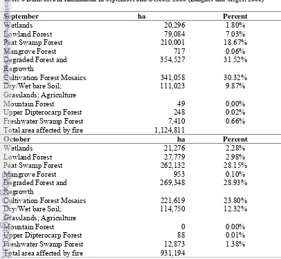
with a value from 1,200 gC m-2 yr-1 to 1,600 gC m-2 yr-1. It was followed by palm oil plantation with NPP of 1,000 gC m-2 yr-1 to 1,300 gC m-2 yr-1. For peatland, the value of NPP varied between 200 gC m-2 yr-1 and 600 gC m-2 yr-1. For water body, the results have shown that NPP varied from 0 gC m-2 yr -1 to 100 gC m-2 yr -1. For residential area, NPP was between 0 gC m-2 yr-1 and 700 gC m-2 yr-1. It increased as long as we got far from the center of the city. In term of mining area, the value of NPP was very low varying between 400 gC m-2 yr-1 to 600 gC m-2 yr-1. This high value might be the result from reforestation and from the vegetation surrounding the mining area since the resolution of the MODIS data used is 250-meter. Geographic and physic condition of the area affected the distribution of NPP. If the region is very mountainous, the value of NPP was very low at about 200 gC m-2 yr-1 and 400 gC m-2 yr-1. However, in the border of Kalimantan, the value of NPP was high reaching 1,400 gC m-2 yr-1 and even 1,800 gC m-2 yr-1. We found out that plenty of forests were still remaining in those areas on the border but we couldn’t verify for the whole area. There was a dramatically drop of NPP in the month of October 2006. It was reported that the 2006 Southeast Asian haze event was caused by continued uncontrolled burning from slash and burn cultivation in Indonesia, and affected several countries in the Southeast Asian region.
The results were validated by doing ground check in three main locations which were South Kalimantan, East Kalimantan, and Central Kalimantan. A sample for water body has been taken on the Mahakam River which is the largest river in East Kalimantan, Indonesia. The sample for forest has been taken in different areas. However, some parts of the very deep forest one was in Tandilang Forest, located in the village called Sulang’ai, Sub-district of Batang Alai Timur, Hulu Sungai Tengah Regency, in South Kalimantan Province. The ground check for peatland was done in a vast peatland area called “Jl Asang Permai Gambut”. The ground check for palm oil was done at the “Kebun Kelapa Sawit Pelaihari”, a palm oil plantation owned by PT. Perkebunan Nusantara XIII (PERSERO). Since it was impossible to go through the mining area, we took the point as close as the mining area as possible and we also took some points from some remaining areas and conditions of previous mining activities. For the residential area, it was done in Pangkalan Bun, capital of the Kotawaringin Barat regency, in the western part of Central Kalimantan.
To improve the prediction of NPP, it is recommended to apply more parameter data such as land cover data from high resolution satellite data. It is important to conduct field experiments and observations for advancing our understanding of the interactions between the carbon and nitrogen cycles in the tropics.
Copyright © 2011, Bogor Agricultural University Copyright are protected by law,
1. It is prohibited to cite all of part of this thesis without referring to and mentioning the source;
a. Citation only permitted for the sake of education, research, scientific writing, report writing, critical writing or reviewing scientific problem. b. Citation does not inflict the name and honor of Bogor Agricultural
University.
NET PRIMARY PRODUCTION SPATIAL DISTRIBUTION
IN KALIMANTAN
SERGE CLAUDIO RAFANOHARANA
A thesis submitted for the degree Master of Science in Information Technology for Natural Resources Management Study Program
GRADUATE SCHOOL
BOGOR AGRICULTURAL UNIVERSITY BOGOR
Research Title : Net Primary Production Spatial Distribution in
Kalimantan
Student Name : Serge Claudio Rafanoharana
Student ID : G051098121
Study Program : Master of Science in Information Technology for
Natural Resources Management
Approved by, Advisory Board
Dr. Ir. Hartrisari Hardjomidjojo, DEA Dr. Ibnu Sofian, M.Eng
Supervisor Co-Supervisor
Endorsed by,
Program Coordinator Dean of the Graduate School
Dr. Ir. Hartrisari Hardjomidjojo, DEA Dr. Ir. Dahrul Syah, M.Sc.Agr
Date of Examination: Date of Graduation:
ACKNOWLEDGMENTS
First and foremost I owe great thanks to God Almighty for bestowing on me the
knowledge and determination to do all the tasks related to this endeavor. He gave
me patience and has always been a generous Guide.
I would like to thank Dr. Ir. Hartrisari Hardjomodjojo, DEA as Program
Coordinator and also my supervisor, Dr. Ibnu Sofian, M.Eng as my co-supervisor
for their guidance, comments, corrections, and constructive inputs through all
months of my research. My appreciation also goes to Prof. Dr. I Nengah Surati
Jaya, M.Agr as the external examiner for his valuable critics, inputs, and
corrections.
I would like to thank the Developing Countries Partnership Scholarship (DCPS)
as my sponsorship during my study here in Indonesia, the administrative staff at
Bogor Agricultural University, and the MIT secretariat for their supports in term
of administration, technical and facility.
I express my thanks to all MIT lecturers who gave me not only knowledge but
also new perspective and vision. Thanks also go to all MIT students for the
togetherness and cultural exchange during our study.
As always, my deepest appreciation goes to my beloved wife Miora Ramilijaona
Rafanoharana for her prayer, love, patience and support during my study. Special
thanks also go to my parents and siblings for their encouragement and support.
Hopefully, the results of this research would provide a positive and valuable
contribution for anyone who reads it.
Bogor, December 2011
CURRICULUM VITAE
The Author was born in Antananarivo, Madagascar on
December 12th 1981. He finished his bachelor degree
in Computer Sciences and Applied Statistics from the
University of Antananarivo, Madagascar. In 2008, he
obtained his Diplôme d'Etudes Superieures
Spécialisées (DESS) in Information System and New
Technology after working for the University of
Antananarivo for two years. He obtained also his
Professional Certificate as a webmaster and web designer from the Conservatoire
National des Arts et Métiers (CNAM) de Paris, France. He obtained a scholarship
from the Developing Countries Partnership Scholarship (DCPS) Program to
pursue his MSc Degree in Information Technology for Natural Resources
Management, an international program under the collaboration of Bogor
Agricultural University and Southeast Asian Regional Centre for Tropical
Biology (SEAMEO BIOTROP). He completed his master program study in 2011.
His final thesis is entitled “Net Primary Production Spatial Distribution in
TABLE OF CONTENTS
Page
TABLE OF CONTENTS... ii
LIST OF TABLES ... iv
LIST OF FIGURES ... v
LIST OF APPENDICES ... vii
I. INTRODUCTION ... 1
1.1 Background ... 1
1.2 Objectives... 2
1.3 Expected Output... 2
II. LITERATURE REVIEW... 3
2.1 Net Primary Production ... 3
2.2 Climate change... 3
2.3 MODIS... 4
III. METHODOLOGY... 5
3.1 Time and Location ... 5
3.2 Required Tools ... 5
3.3 Data Source ... 5
3.4 Method ... 6
3.4.1 Data collection ... 6
3.4.2 Data Processing... 7
3.4.3 Measuring vegetation: Enhanced Vegetation Index (EVI) ... 8
3.4.4 Estimation of Net Primary Production (NPP)... 9
3.4.5 Validation with the ground check ... 12
IV. RESULTS ... 16
4.1 Enhanced Vegetation Index (EVI) ... 16
4.1.1 Climatology process and Anomalies of EVI... 17
4.1.2 Spatial distribution of Enhanced Vegetation Index ... 18
4.2 Temperature ... 20
4.3 Precipitation ... 22
4.4 Fraction of Absorbed Photosynthetically Active Radiation (FPAR).... 24
4.5 Net Primary Production (NPP) ... 27
4.5.1 Monthly mean of NPP... 27
4.5.2 Yearly mean of NPP... 28
4.5.3 Climatology Process and Anomalies of NPP... 29
4.5.4 Correlation of NPP with Climate Variability... 32
4.5.5 Spatial distribution of NPP in Kalimantan... 35
4.6 Validation... 39
4.6.1 Ground check for water body... 40
4.6.2 Ground check for forest ... 41
4.6.3 Ground check for Peatland... 43
4.6.4 Ground check for Palm Oil ... 43
4.6.5 Ground check for Mining area ... 45
4.6.6 Ground check for Residential area... 45
V. CONCLUSION AND RECOMMENDATION ... 47
5.1 Conclusion ... 47
5.2 Recommendation ... 48
REFERENCES... 49
APPENDICES ... 53
LIST OF TABLES
Page
Table 1 The general pattern of monthly EVI in Kalimantan ... 19
Table 2 The general pattern of monthly Temperature in Kalimantan... 22
Table 3 The general pattern of monthly Precipitation in Kalimantan (in mm)... 24
Table 4 The general pattern of monthly FPAR in Kalimantan ... 26
Table 5 The general pattern of monthly NPP in Kalimantan... 31
Table 6 Burnt area in Kalimantan in September and October 2006 (Langner and Siegert 2006) ... 38
LIST OF FIGURES
Page
Figure 1 Location of the study area... 5
Figure 2 General Method of the Research ... 7
Figure 3 Time series of monthly mean of EVI in Kalimantan... 16
Figure 4 Time series of monthly mean of EVI and monthly average of 10-year period ... 17
Figure 5 Time series of anomalies for EVI from 2001 to 2010 ... 18
Figure 6 Yearly mean of EVI in the year 2001, 2005, 2006, and 2010 ... 20
Figure 7 Monthly average temperature over Kalimantan from 2001 to 2010 ... 21
Figure 8 Monthly average precipitation over Kalimantan from 2001 to 2010 ... 23
Figure 9 Time series of FPAR over Kalimantan from 2001 to 2010... 25
Figure 10 Trends of monthly distribution of NPP in Kalimantan... 27
Figure 11 Trends of annual distribution of NPP in Kalimantan ... 28
Figure 12 Time series of monthly mean of NPP and monthly average of 10-year period ... 29
Figure 13 Time series of anomalies of NPP from 2001 to 2010... 30
Figure 14 Time series data of NPP and Temperature in Kalimantan ... 32
Figure 15 Correlation between NPP and Temperature data in Kalimantan... 33
Figure 16 Time series data of NPP and Precipitation in Kalimantan ... 34
Figure 17 Correlation between NPP and Precipitation data in Kalimantan... 34
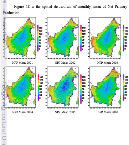
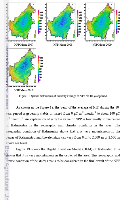
Figure 18 Spatial distribution of monthly average of NPP for 10-year period... 36
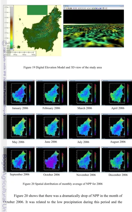
Figure 19 Digital Elevation Model and 3D view of the study area ... 37
Figure 20 Spatial distribution of monthly average of NPP for 2006 ... 37
Figure 21 Location for ground check and validation of NPP ... 40
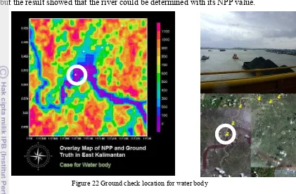
Figure 22 Ground check location for water body ... 41
Figure 23 Ground check location for forest (a)... 41
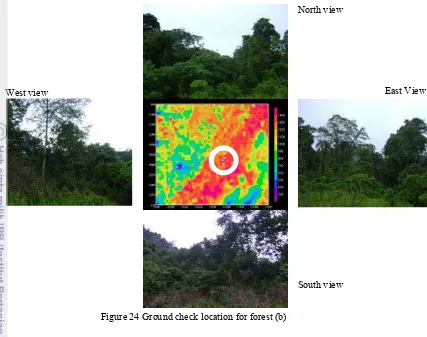
Figure 24 Ground check location for forest (b) ... 42
Figure 25 Forest Map of South Kalimantan... 42
Figure 26 Ground check location for peatland... 43
Figure 27 Ground check location for palm oil plantation (a)... 44
Figure 28 Ground check location for palm oil plantation (b) ... 44
Figure 29 Ground check location for mining area ... 45
Figure 30 Ground check location for residential area... 46
vii
LIST OF APPENDICES
Page 1 Batch file program for data processing ... 53
I. INTRODUCTION
1.1 Background
Temperature of the Earth is controlled by the balance between the input
from energy of the sun that hits the earth and the loss of this energy reflected back
into space. On average, about one-third of the solar radiation is reflected back to
space. Of the remainder, some is absorbed by the atmosphere, but most is
absorbed by the land and oceans (Maslin 2004). Certain atmospheric gases are
critical to the temperature balance and are known as greenhouse gases. The
existence of greenhouse gases includes water vapor, carbon dioxide, ozone,
methane, and nitrous oxide could a blanket effect and would increase the
temperature of the earth. Global temperatures have risen by 0.76oC since 1850,
with doubled warming rate compare to the past century (Partington 2007).
The increasing concentration of atmospheric greenhouse gases could also
threatened the existence of human beings. Understanding the response of
ecosystem to climate change would be necessary for human beings to protect the
environment and for the production of food and energy. Vegetation could act as
carbon source or sink to greenhouse gases (Schimel et al. 2000, Braswell et al.
1997). According to Partington (2007) and also Dutschke and Wolf (2007), it was
mentioned that deforestation is considered as the second most important
human-induced source of greenhouse gases. This was being responsible for
approximately 20% of total emissions. Much knowledge has been gathered on
drivers and causes of deforestation and forest degradation at recent years, also
methodological tools have been developed to monitor large areas and predict the
quantification of carbon benefits from reduced deforestation and forest
degradation (REDD).
Net Primary Production (NPP) is defined as the net flux of carbon from the
atmosphere into green plants per unit time (Zhiqiang et al. 2004). Annual NPP is
the net amount of carbon captured by land plants through photosynthesis each
year. Studying the response of NPP to the environment could help understand the
functions of ecosystem and its feedback to the changes of climate and social
utilization and development of agriculture and forestry (Lobell et al. 2002,
Mingkui and Woodward 1998). Net Primary Production of terrestrial ecosystems
is important in estimating land carrying capacity, which is critically relevant to the
social and economic development of a country. An objective and critical review of
past efforts to estimate forest NPP calls into question the precision and accuracy
of such estimates (Clark et al. 2001), new techniques such as eddy flux correlation
(Goulden et al. 1996) and more explicit identification of NPP components (Clarck
et al. 2001) have led to improved estimates. Temporal trends lead to differences in
estimated NPP and its allocation, depending on stand age or development stage
(Kira 1975); hence, comparisons among species of forest types must be done with
some caution.
MODIS data could be used to estimate the spatial distribution of NPP.
MODIS offers a unique combination of features such as detection of a wide
spectral range of electromagnetic energy; measurement at three spatial resolutions
and time of measurements take in place. These advantages allowed MODIS to
complete an electromagnetic picture of the globe every two days. MODIS’
frequent coverage could complement other imaging systems such as Landsat’s
Enhanced Thematic Mapper Plus, which reveals the Earth in finer spatial detail,
but can only image a given area once every 16 days. The research is aimed to
estimate the NPP using MODIS for Kalimantan area.
1.2 Objectives
The objectives of this research are:
- to estimate the Net Primary Production (NPP) using Moderate Resolution
Imaging Spectroradiometer (MODIS) Enhanced Vegetation Index (EVI)
- to validate the estimation of NPP with the ground check
1.3 Expected Output
The expected output is the estimation of the total Net Primary Production,
based on MODIS data in Kalimantan during 2001 to 2010. We also expect to
obtain the spatial distribution of NPP, and validate the estimation with the ground
II. LITERATURE REVIEW
2.1 Net Primary Production
NPP is a measurement of plant growth obtained by calculating the quantity
of carbon absorbed and stored by vegetation. NPP is equal to photosynthesis
minus respiration. It is sometimes expressed in grams of carbon per square meter
per year. It is a major component of the carbon cycle. Net primary productivity
(NPP) is also defined as the net flux of carbon from the atmosphere into green plants
per unit time. NPP refers to a rate process, i.e., the amount of vegetable matter
produced (net primary production) per day, week, or year. It is a tool for measuring
forest productivity and establishing carbon budgets. The data obtained by
calculating NPP can be used as the basis for estimating the impact of both natural
disturbances and management activities on forest productivity, assessing the
effects of climate change on forests, and assessing the role that these forests can
play in achieving our greenhouse-gas reduction objectives (Lobell et al. 2002,
Mingkui and Woodward 1998). MODIS NPP is an annual value and provides a
means of evaluating spatial patterns in productivity as well as interannual
variation and long term trends in biosphere behavior (Turner et al. 2006).
2.2 Climate change
Plants capture and store solar energy through photosynthesis. During
photosynthesis, living plants convert carbon dioxide in the air into sugar
molecules they use for food. In the process of making their own food, plants also
provide the oxygen that is very important for human beings. Plant productivity
also plays a major role in the global carbon cycle by absorbing some of the carbon
dioxide released from the people activities sech as burning coal, oil, and other
fossil fuels. The carbon plants absorbed would becomes part of leaves, roots,
stalks or tree trunks, and ultimately, the soil.
Climate change is a long-term change in the statistical distribution of
weather patterns over periods of time that range from decades to millions of years.
It may cause a change in the average weather conditions for example greater
affected the climate are climate forcing such variations in solar radiation,
deviations in the earth's orbit, and changes in greenhouse gas concentrations.
There are a variety of climate change feedbacks that can either amplify or
diminish the initial forcing. Some parts of the climate system, such as the oceans
and ice caps, respond slowly in reaction to climate forcing because of their large
mass. Therefore, the climate system can take centuries or longer to fully respond
to new external forcing.
2.3 MODIS
MODIS (or Moderate Resolution Imaging Spectroradiometer) is a key
instrument aboard the Terra (EOS AM) and Aqua (EOS PM) satellites. Terra's
orbit around the Earth is timed so that it passes from north to south across the
equator in the morning, while Aqua passes south to north over the equator in the
afternoon. Terra MODIS and Aqua MODIS are viewing the entire Earth's surface
every 1 to 2 days, acquiring data in 36 spectral bands, or groups of wavelengths.
These data improved our understanding of global dynamics and processes
occurring on the land, in the oceans, and in the lower atmosphere. MODIS is
playing a vital role in the development of validated, global, interactive Earth
system models to predict global change accurately enough to assist policy makers
in making sound decisions concerning the protection of our environment.
The pair of Vegetation Indices from MODIS data highlights some of the
refinements of the MODIS Enhanced Vegetation Index (EVI, right) over the
traditional Normalized Difference Vegetation Index (NDVI, left) that has been
used with previous satellite instruments. NDVI tends to “saturate” over dense
vegetation such as the rainforests of South America, failing to distinguish
variability. The MODIS EVI provides a more detailed look at variability within
such highly vegetated regions. Production of MODIS NDVI provides continuity
with data sets from heritage instruments, while EVI provides detail of global
vegetation variability. Neither the NDVI nor the EVI product eliminated all
obstacles. Clouds and aerosols can often block the satellites’ view of the surface
entirely, glare from the sun can saturate certain pixels, and temporary
III. METHODOLOGY
3.1 Time and Location
The research was conducted from March until October 2011. The study area
was Kalimantan which is bounded between longitude 108o 40’ 58’’ E and 118o
59’ 45’’ E and latitude 4o 24’ 8’’ N and 4o 22’ 30’’ S with an area of
approximately 537.442,55 km2. The Figure 1 shows the area of study (inside the
red boundary).
Figure 1 Location of the study area
3.2 Required Tools
One of the important steps for the study is the selection of the appropriate
software. For that, we used GRADS 2.0 and MODIS Tool. In addition,
appropriate hardware selection is also important so that its compatibility with the
selected software might not cause any problem during all processes. Computers
supported with high-speed Internet connection were required for this research.
The research was done at the laboratory of Master of Science in Information
Technology for Natural Resources Management (M.Sc. in IT for NRM) at
SEAMEO BIOTROP.
3.3 Data Source
MODIS satellite data was used for this research. The data was collected
starting from the year 2001 to 2010. MOD13Q1 type in a Terra platform was used
of 250m and a temporal granularity of 16 days. In addition, FPAR data was
downloaded from 2001 to 2010.
MODIS might be so far, the most complex instrument built and flown on a
spacecraft for civilian research purposes. The MODIS sensor provides higher
quality data for monitoring terrestrial vegetation and other land processes than the
previous AVHRR, not only because its narrower spectral bands that enhance the
information derived from vegetation, but also because leading scientists are
working as a team to improve the accuracy of the data from low level reflectance
data, to high level data, such as land cover, fire, land surface temperature,
vegetation indices (NDVI and EVI; EVI is the enhanced vegetation index), FAPR
/ LAI and GPP / NPP (Justice et al. 2002)
3.4 Method
3.4.1 Data collection
MODIS data was used for this study. We login the MODIS/Terra Multiple
Data Ordering Page to download MODIS data for our study sites. Since
Kalimantan has a wide area, it could not be covered by one single image of
MODIS data. In order to cover the whole area of Kalimantan, the MODIS data
could be downloaded in a tile fashion, from which each tile covers approximately
10 latitude by 10 longitude.
For Kalimantan area, four images MODIS data was needed for EVI.
MODIS Tool and GRADS 2.0 were the software used to process MODIS data.
MODIS EVI
Data Processing
Estimation of EVI
Spatial Distribution of NPP
Validation
Recommendation Mosaicking
End Start
Ground check
Figure 2 General Method of the Research
3.4.2 Data Processing
There was several remote sensing techniques applied in this research. The
first step of the work was mosaicking the images. This was done by using MODIS
non geo referenced images within a mosaic, and automated placement of geo
referenced images within a geo referenced output mosaic and conduct the other
data processing. The same process was done for MODIS EVI and other data.
3.4.3 Measuring vegetation: Enhanced Vegetation Index (EVI)
In December 1999, NASA launched the Terra spacecraft, the flagship in
the agency’s Earth Observing System (EOS) program. Aboard Terra flies a sensor
called the Moderate-resolution Imaging Spectroradiometer, or MODIS, that
greatly improves scientists’ ability to measure plant growth on a global scale.
MODIS provides much higher spatial resolution (up to 250-meter resolution),
while also matching Advanced Very High Resolution Radiometer (AVHRR)’s
almost-daily global cover and exceeding its spectral resolution. In other words,
MODIS provided images over a given pixel of land just as often as AVHRR, but
in much finer detail and with measurements in a greater number of wavelengths
using detectors that were specifically designed for measurements of land surface
dynamics.
Consequently, the MODIS Science Team prepared a new data product–
called the Enhanced Vegetation Index (EVI) that improved upon the quality of the
NDVI product. The EVI took full advantage of MODIS’ new, state-of-the-art
measurement capabilities. The EVI is calculated similar to NDVI, but with
corrections for some distortions in the reflected light caused by the particles in the
air as well as the ground cover below the vegetation. The EVI data product also
does not become saturated as easily as the NDVI when viewing rainforests and
other areas of the Earth with large amounts of chlorophyll.
Vegetation indices derived from remote sensing data provide information
about consistent, spatial and temporal comparisons of global vegetation conditions
which was used to monitor the Earth's terrestrial photosynthetic vegetation
activity. For example, the enhanced vegetation index (EVI) provides a measure of
greenness of the vegetation that can be used to predict net primary production.
The Enhanced Vegetation Index (EVI) improves on the venerable NDVI.
Derived from state-of-the-art satellite data provided by the MODIS instrument,
heavily vegetated areas. The EVI is related to the optical measures of vegetation, a
direct measure of photosynthetic potential resulting from composite chlorophyll,
leaf area, canopy cover, and structure. It is developed to optimize the vegetation
signal with improved sensitivity in high biomass regions and improved vegetation
monitoring through a de-coupling of the canopy background signal and a
reduction in atmosphere influences. The equation takes the form,
EVI = G * (ρNIR – ρRed) / (ρNIR + C1 * ρRed – C2 * ρBlue + L)
Where,
EVI = Enhanced Vegetation Index
G = Gain factor (=2.5)
ρNIR = Near Infrared Reflectance
ρRed = Red Reflectance
ρBlue = Blue Reflectance
C1 = Atmosphere Resistance Red Correction Coefficients (=1)
C2 = Atmosphere Resistance Blue Correction Coefficients (=6.0)
L = Canopy Background Brightness Correction Factor (=1)
The input reflectance to the EVI equation may be
atmospherically-corrected or partially atmosphere atmospherically-corrected for Rayleigh scattering and ozone
absorption. C1 and C2 are the coefficients of the aerosol resistance term, which
uses the blue band to correct for aerosol influences in the red band. The canopy
background adjustment factor, L, addresses non-linear, differential NIR and red
radiant transfer through a canopy and renders the EVI insensitive to most canopy
backgrounds, with snow backgrounds as the exception.
3.4.4 Estimation of Net Primary Production (NPP)
This estimation was based on the value of EVI. The methods for
measurement of primary production vary depend on the focus that we would like
to calculate, the gross or net production, terrestrial or aquatic system. The
production of plant biomass (Potter et al. 2009) which is estimated as a product of
time varying surface solar irradiance and EVI from the MODIS satellite, with a
constant light utilization efficiency term that is modified by time varying stress
scalar terms for temperature and moisture effects. As documented in Potter (1999),
the monthly NPP flux, defined as net fixation of CO2 by vegetation, is computed
in NASA–CASA on the basis of light-use efficiency (Monteith 1972). Monthly
production of plant biomass is estimated as a product of time-varying surface
solar irradiance (Sr) (Kistler et al. 2001), and EVI from the MODIS satellite
(Huete et al., 2002), and a constant light utilization efficiency term (emax) that is
modified by time-varying stress scalar terms for temperature (T) and moisture (W)
effects. The equation to estimate the NPP is defined below.
NPP = Sr EVI emax Tscalar Wscalar
Where,
NPP = Net Primary Production (gC m-2 year-1)
Sr = Solar irradiance (W m-1)
EVI = Enhanced Vegetation Index from MODIS
emax = Constant Light Utilization Efficiency Term
Tscalar = Optimal temperature for plant production
Wscalar = Monthly water deficit
The emax term is set uniformly at 0.39 gC MJ−1 PAR, a value that derives from calibration of predicted annual NPP to previous field estimates (Potter et al.
1993). Tscalar is computed with reference to derivation of optimal temperatures
(Topt) for plant production. Topt setting varied by latitude and longitude, ranging
from near 0°C in the Arctic to the middle thirties in low-latitude deserts. Wscalar is
estimated from monthly water deficits, based on a comparison of moisture supply
(precipitation and stored soil water) to potential evapotranspiration (PET).
The PAR values are actually restricted to just a portion of electromagnetic
light of human eye can see. Therefore, this value was assumed to be
approximately 0.5 of the incoming solar radiation (Rasib et al. 2008) and it was
used for this research.
Tscalar is estimated using the equation developed for the terrestrial ecosystem
model (Raich et al. 1991). The equation for Tscalar is:
Tscalar = [ (T – Tmax) (T – Tmin) ] / [ (T – Tmax) (T – Tmin) – (T – Topt)2 ]
where T is the observed temperature (oC) and Tmin, Tmax, and Topt are minimum,
maximum, and optimal temperature for photosynthesis with a value of 20oC, 40oC,
and 30oC respectively.
Wscalar is the effect of water deficit on plant photosynthesis, and is
estimated as a function of rainfall, run off, groundwater reserves and potential
evapotranspiration. The equation for Wscalar is defined below:
Wscalar = 0.5 + [ 0.5 * (EET / PET) ]
where EET and PET are estimated and potential evapotranspiration, where Wscalar
ranged between 0.5 (dry) to 1 (wet). Therefore, the function in Wscalar can be
described as below:
PPT > PET => EET = PET
PPT < PET => EET = PPT
where PPT is the total precipitation. Water run-off and groundwater reserves are
ignored and where PET is calculated based on Priestley and Taylor (1972) with
the equation:
where Rn is the net-radiation (MJ m-2 month-1), G is the heat flux at ground level
assumed to be 0, γ is the constant psychometric with a value of about 66 Pa K-1.
and α are the latent heat of evaporation and the empirical factor of with values 2.5
MJ Kg-1 and 1.26 respectively. Δ is calculated using the following mathematical
equation:
Δ = 2504 * exp [(17.27 * T) / (T + 237.2)] / (T + 237.3)2
where Δ is the slope vapour pressure curve (KPa oC-1) and T the air temperature
(oC).
3.4.5 Validation with the ground check
The result of the calculation should be validated with the ground check.
Validation of the NPP is an essential step in establishing its utility; however,
validation is challenging because of a variety of scaling issues (Morisette et al.
2002, Turner et al. 2004). Site-level validation of MODIS NPP has been more
limited because of the logistical constraints of measuring NPP and scaling it to the
size of a MODIS grid cell (Turner et al. 2004, 2005). These efforts have likewise
found site-specific differences in the degree of agreement between ground-based
and MODIS-based NPP estimates. The MODIS NPP algorithm requires the
computation of autotrophic respiration (Ra) based on inputs of leaf area index
(LAI) and temperature, along with look-up table values for constants and the base
rate of respiration (Running et al. 2000). Specific problems with the Ra
component of NPP have been identified in some cases (Turner et al. 2005).
It is widely known that tower flux measurements of Net Ecosystem
Production (NEP) can be used for model validation at the small site scale.
Nevertheless, we have not included comparisons of tower-based NEP to
NASA-CASA modeled NEP in this island study, because tower eddy flux estimates are
not designed to represent large-scale (e.g., 8 km) NEP fluxes that we model with
NASA-CASA.
NEP is named ecosystem carbon sink (positive value) or carbon source
release. Theoretically, when an ecosystem matures, e.g. climax, it is in
equilibrium with the climate and soil environment, so the carbon uptake and
release are balanced, and NEP approximates to zero. But if the environmental
conditions, such as climate, changed, the ecosystem carbon budgets were not
balanced.
In any year over the past nine years, net ecosystem production can be very
large in one location but very small or negative in another location because of the
spatial heterogeneity of vegetation, soils and climate. Locations with large
positive annual NEP are often those that receive a high amount of precipitation. In
contrast, locations with negative NEP are often those that receive little
precipitation. Year-to-year changes in spatial pattern of NEP were most probably
caused by changes in the spatial pattern of precipitation, which can be changed
dramatically by the El Nino events (Vörösmarty et al. 1996).
For this research, different samples from different areas for ground check
were considered. The first area was related to the place where the highest value of
NPP is found. The second area was a place where the lowest value of NPP is
found. For that, we checked on the ground what kind of features exists exactly in
the area, and how can we come up with a conclusion based on what we found in
the area with our system.
A sample for water body has been taken on the Mahakam River which is
the largest river in East Kalimantan, Indonesia, with a catchment area of
approximately 77,100 km2. The catchment lies between 2˚N to 1˚S latitude and
113˚E to 118˚E longitude. The river originates in Cemaru (Van Bemmelen 1949)
from where it flows south-eastwards, meeting the River Kedang Pahu at the city
of Muara Pahu. From there, the river flows eastward through the Mahakam lakes
region, which is a flat tropical lowland area surrounded by peat land. Thirty
shallow lakes are situated in this area, which are connected to the Mahakam
through small channels.
The samples for forests have been taken in different areas. However, some
parts of the very deep forest one was in Tandilang Forest, located in the village
called Sulang’ai, Sub-district of Batang Alai Timur, Hulu Sungai Tengah Regency,
Over the past decade, the government of Indonesia has drained some peat
swamp forests of the island of Borneo for conversion to agricultural land. The dry
years of 1997-8 and 2002-3 saw huge fires in the peat swamp forests. A study for
the European Space Agency found that the peat swamp forests are a significant
carbon sink for the planet, and that the fires of 1997-8 may have released up to 2.5
billion tonnes, and the 2002-3 fires between 200 million to 1 billion tonnes, of
carbon into the atmosphere. Much of the emissions from peatlands in Borneo are
due to changes in their hydrological regime, caused by drainage from nearby
plantations (particularly oil palm). Peatland conservation and rehabilitation are
more efficient undertakings than reducing deforestation (in terms of claiming
carbon credits from REDD initiatives), due to the much larger reduced emissions
achievable per unit area and the much lower opportunity costs involved (Mathai
2009). Indonesia contributes 50 percent of tropical peat swamps and 10 percent of
dry land in the world. The ground check for peatland was done in a vast peatland
area called “Jl Asang Permai Gambut”.
Deeper analysis in Indonesia suggests that oil palm development might be
a cover for something more lucrative: logging. Recently much has been made
about the conversion of Asia's biodiversity rainforests for oil-palm cultivation.
Environmental organizations have warned that by eating foods that use palm oil as
an ingredient, Western consumers are directly fueling the destruction of orangutan
habitat and sensitive ecosystems. However, oil-palm plantations now cover
millions of hectares across Malaysia, Indonesia, and Thailand.
Palm oil became the world's number one fruit crop, trouncing its nearest
competitor, the humble banana because of its crop's unparalleled productivity.
Palm oil is the most productive oil seed in the world. A single hectare of oil palm
may yield 5,000 kilograms of crude oil, or nearly 6,000 liters of crude. The
ground check for palm oil was done at the “Kebun Kelapa Sawit Pelaihari”, a
palm oil plantation owned by PT. Perkebunan Nusantara XIII (PERSERO).
Mining sector in South Kalimantan Province is dominated by oil, natural
gas and coal, but oil and natural gas is inclined to have decreased, coal precisely
have very fast increasing amount. Coal has been blamed as a major contributor to
abundant deposits of coal and contributes 16.36 % to the national coal stock. Coal
mining is a profitable business. It creates employment, generates value, and
improves the foreign investment of a country or region. However, coal mining has
its disadvantages including not to mention the impact to the environment. Since it
was impossible to go through the mining area, we took the points as close as the
mining area as possible and we also took some points from some remaining areas
and conditions of previous mining activities.
For residential area, the ground check was done in Pangkalan Bun, capital
of the Kotawaringin Barat regency, in the western part of Central Kalimantan.
This is the entry point to reach Tanjung Puting Park in the southern part, and the
IV. RESULTS
4.1 Enhanced Vegetation Index (EVI)
The enhanced vegetation index (EVI) was developed to optimize the
vegetation signal with improved sensitivity in high biomass regions and improved
vegetation monitoring through a de-coupling of the canopy background signal and
a reduction in atmosphere influences. In this study, the Enhanced Vegetation
Index data were obtained from MODIS. Low EVI is sparsely vegetated land, high
EVI is densely vegetated land, and EVI where values are equal to or below zero
are assumed to be typically caused by water bodies.
EVI
Figure 3 Time series of monthly mean of EVI in Kalimantan
Figure 3 illustrates changes in the average value of EVI in Kalimantan
between 2001 and 2010. In October 2005, the amount of EVI reached its highest
amount with about 0.55, while the lowest amount was in October 2006, around
0.46. However, during this 10-year period, there were a lot of changes to the
proportion of EVI. In the beginning of 2001, the value was about 0.51 then 0.55 in
March 2001, but a dramatic fall was noticed in November 2002 (around 0.48). A
big variation was seen until July 2005: the EVI varied between 0.49 and 0.53. On
the other hand, a small variation was noticed over the next five years (2006-2010).
The value of EVI reached its peak in March 2006, September 2007, March 2008,
and September 2010 with a value of 0.53, 0.52, 0.53, and 0.52 respectively.
However, it decreased rapidly to 0.46 by the end of 2010. Overall, Figure 3 shows
4.1.1 Climatology process and Anomalies of EVI
Figure 4 Time series of monthly mean of EVI and monthly average of 10-year period
Figure 4 compares the monthly mean of EVI and the Climatology Process
in Kalimantan for 10 years. As can be seen in Figure 4, the proportion of EVI
varied between around 0.46 to 0.55 while the monthly average of 10 years was
around 0.49 to 0.54. In the beginning of 2001, the monthly average of 10 years
was by far lower than the proportion of EVI: it was only about 0.52 while the EVI
was about 0.54. However, at mid-2001, the amount of EVI declined dramatically
to almost 0.50 which was almost similar to the monthly average of 10 years.
During the 10-year period, the proportion of EVI varied a lot. In general, the value
was more than 0.50 except at the end of 2002 and 2006, from the middle of 2009
until mid-2010, and by the end of 2010. The monthly average of 10 years for EVI,
on the other hand, showed a small variation. Even if there are many upward and
downward trends happening throughout the period, the value was not lower than
0.49. Overall, Figure 4 showed that the proportion of EVI was much more stable
from 2001 to mid 2009 except in October 2006 and was quite low from mid-2009
b. Anomalies
Figure 5 Time series of anomalies for EVI from 2001 to 2010
Figure 5 shows the anomalies for the EVI in Kalimantan from 2001 to
2010. It is clear that the values varied between -0.04 and 0.05 during this 10-year
period. In October 2005, it reached its peak with a value of 0.05, whereas in
October 2006, it had its lowest value at -0.04. For the other years, the variation
was around -0.03 to 0.02. During the first 5 years, all values are positive except in
September to December 2002, April 2003, and August 2004 to June 2005, where
the variation of the anomalies showed a downward trend. Similarly a downward
trend was also noticed over the last 5-year period. However, some of the values
are above 0 in February to June 2006, January and May 2007, September 2007 to
March 2008, August to December 2008, February and April 2009, and September
to November 2010 before a rapid decline by the end of 2010 with a value of -0.03.
Overall, Figure 5 indicates that there was a difference between the variations of
the values of the anomalies of EVI from 2001 to 2005, and from 2006 to 2010.
4.1.2 Spatial distribution of Enhanced Vegetation Index
Enhanced Vegetation Index (EVI) data were obtained from the MODIS
sensor. It corrects for some distortions in the reflected light caused by the particles in
the air as well as the ground cover below the vegetation. The EVI data product also
does not become saturated as easily as NDVI when viewing rainforests and other area
of the Earth with large amounts of chlorophyll. The EVI data are designed to provide
the potential for regional analysis and systematic and effective monitoring of the
forest area.
The EVI values were resulted from 10-year estimation. The values vary
between -0.2 as minimum to 1 as maximum. The EVI values equal to or below zero
were assumed to be typically caused by water bodies. The low EVI values were
sparsely vegetated land meanwhile the high EVI values were densely vegetated land.
Estimation of EVI values over Kalimantan terrestrial from 2001 to 2010 are shown in
the Table 1.
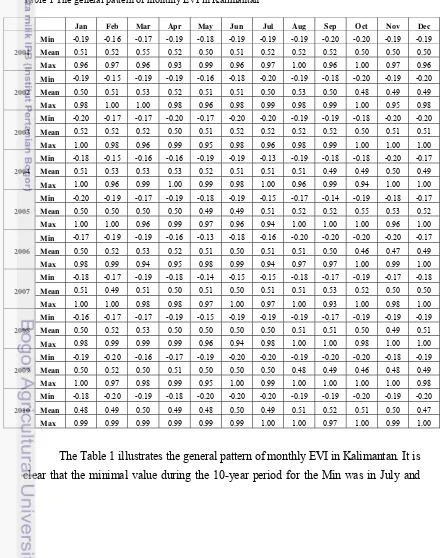
Table 1 The general pattern of monthly EVI in Kalimantan
Jan Feb Mar Apr May Jun Jul Aug Sep Oct Nov Dec
The Table 1 illustrates the general pattern of monthly EVI in Kalimantan. It is
September of 2001 and 2009 with a value of about -0.20; while the maximal value for
the Min was in May and July 2004 with a value of about -0.12. The Mean had its
highest value in October 2005 with about 0.55; and its lowest amount in October
2006 with 0.45. For the Max, the October 2005 proportion about 1 was the highest
throughout the 10-year period; whereas the September 2007 with about 0.92 was the
lowest.
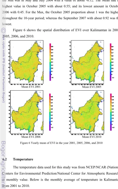
Figure 6 shows the spatial distribution of EVI over Kalimantan in 2001,
2005, 2006, and 2010.
Mean EVI 2001 Mean EVI 2005
Mean EVI 2006 Mean EVI 2010 Figure 6 Yearly mean of EVI in the year 2001, 2005, 2006, and 2010
4.2 Temperature
The temperature data used for this study was from NCEP/NCAR (National
Centers for Environmental Prediction/National Center for Atmospheric Research)
at monthly value. Below is the monthly average of temperature in Kalimantan
TEMP
Figure 7 Monthly average temperature over Kalimantan from 2001 to 2010
Figure 7 gives information about changes of the monthly average
temperature in Kalimantan between 2001 and 2010. The monthly average
temperature in Kalimantan ranged between 25.04°C to 26.38°C except in May
2010 where it reached 26.72°C. The pattern of monthly average temperature
showed that monthly average temperature in Kalimantan reached its highest
temperature value during May and June. It is evident that the value of monthly
average temperature in Kalimantan decreased from November to February for
every year from about 25.7°C to 25.1°C. Similarly in July of every year, it fell
slightly from about 25.9°C to 25.4°C; and for the other period of the year
especially from February to May, the figure showed an upward trend with a value
of about 25.05°C to 26.3°C and reached its peak in May or June. The monthly
average temperature had its highest value in May 2010 and its lowest value in
January 2009 with a value of 26.72°C and 25.04°C respectively. In general, each
year variation’s trend was almost the same over the 10-year period from 2001 to
2010.
Table 2 reveals the general pattern of monthly temperature in Kalimantan
from 2001 to 2010. It is showed that for the Min, the highest value was in May
Table 2 The general pattern of monthly Temperature in Kalimantan
Jan Feb Mar Apr May Jun Jul Aug Sep Oct Nov Dec Min 21.87 21.93 22.04 22.08 22.04 21.55 21.30 21.28 21.52 21.87 21.62 21.43
2001 Mean 25.50 25.37 25.79 26.15 26.38 26.09 25.81 25.93 25.77 26.00 25.83 25.39
Max 27.92 27.79 28.04 28.80 29.39 29.22 29.13 29.42 28.48 28.34 28.23 27.87
Min 21.58 21.52 21.80 21.95 22.07 21.66 21.16 20.92 21.19 21.53 21.71 21.79
2002 Mean 25.22 25.06 25.44 25.94 26.27 26.05 25.90 25.69 25.54 25.79 25.91 25.90
Max 28.03 27.88 28.09 28.37 29.20 29.32 29.50 29.16 28.58 28.28 28.37 28.59
Min 21.72 21.57 21.75 22.11 21.77 21.46 21.26 21.40 21.43 21.82 21.68 21.68
2003 Mean 25.48 25.24 25.54 26.08 26.26 25.81 25.70 25.80 25.86 25.91 25.78 25.39
Max 28.17 27.98 28.06 28.54 29.38 28.89 28.86 29.14 29.00 28.43 28.08 27.79
Min 21.68 21.64 21.99 22.10 21.92 21.11 21.26 20.74 21.30 21.37 21.67 21.69
2004 Mean 25.18 25.10 25.60 26.17 26.30 25.96 25.45 25.54 25.43 25.66 25.71 25.50
Max 27.87 27.86 28.03 28.76 29.45 29.67 28.49 29.28 28.27 28.24 28.19 28.01
Min 21.61 21.68 21.85 22.10 22.26 21.88 21.71 21.41 21.52 21.86 21.84 21.86
2005 Mean 25.06 25.31 25.54 25.93 26.33 26.36 25.98 25.85 26.00 26.02 25.86 25.68
Max 27.69 27.96 28.32 28.38 29.23 29.64 29.21 29.04 29.10 28.45 28.12 28.29
Min 21.81 22.02 21.94 22.04 21.99 21.70 21.58 21.25 21.45 21.78 21.66 22.17
2006 Mean 25.21 25.38 25.56 25.87 26.10 25.87 25.93 25.79 25.63 25.75 25.70 25.90
Max 27.71 27.75 27.89 28.27 28.97 28.91 29.25 29.16 28.41 28.20 28.26 28.23
Min 22.06 21.90 22.03 22.28 22.21 22.08 21.62 21.38 21.52 21.86 21.60 21.96
2007 Mean 25.44 25.13 25.55 25.91 26.14 26.14 25.80 25.62 25.74 25.76 25.45 25.50
Max 28.02 27.54 27.75 28.24 28.79 29.23 29.03 28.86 28.62 28.09 27.54 28.03
Min 21.64 21.73 21.78 22.08 21.88 21.81 21.43 21.52 21.79 21.93 22.04 21.97
2008 Mean 25.18 25.06 25.20 25.78 25.95 25.79 25.47 25.52 25.86 25.87 25.89 25.59
Max 27.45 27.57 27.43 28.11 28.61 28.66 28.47 28.30 28.71 28.41 28.09 28.00
Min 21.60 21.83 21.82 22.06 22.20 21.65 21.49 21.70 21.84 21.92 21.91 21.88
2009 Mean 25.05 25.18 25.55 26.21 26.34 26.15 25.95 25.90 26.04 25.88 25.90 25.55
Max 27.43 27.60 27.70 28.78 29.01 29.43 29.24 28.79 28.82 28.24 28.38 27.97
Min 21.65 22.07 22.27 22.59 22.68 22.13 21.92 21.78 21.78 22.01 21.84 21.67
2010 Mean 25.40 25.58 25.83 26.39 26.73 26.37 26.01 25.95 25.96 26.08 25.84 25.39
Max 27.84 28.07 28.17 28.76 29.43 29.45 28.87 28.84 28.66 28.55 28.22 27.80
The value of Mean, on the other hand, reached its highest proportion in
May 2010 and its lowest proportion in January 2009 with about 26.72 oC and
25.04 oC respectively. The Max, however, had its maximal temperature in June
2004 with 29.67 oC and its minimal temperature in February 2008 with 27.43 oC.
4.3 Precipitation
The Tropical Rainfall Measuring Mission (TRMM) is a joint U.S.-Japan
satellite mission to monitor tropical and subtropical precipitation and to estimate
its associated latent heating. TRMM was successfully launched on November 27,
measuring instruments on the TRMM satellite include the Precipitation Radar
(PR), an electronically scanning radar operating at 13.8 GHz; TRMM Microwave
Image (TMI), a nine-channel passive microwave radiometer; and Visible and
Infrared Scanner (VIRS), a five-channel visible/infrared radiometer. TRMM data
was used in order to derive the precipitation.
PRE
Figure 8 Monthly average precipitation over Kalimantan from 2001 to 2010
The Figure 8 reveals the monthly average precipitation in Kalimantan over
10-year period from 2001 to 2010. Monthly Average precipitation varied from 44
mm to 376 mm per month. The highest precipitation was found during the months
of December and January. At the beginning of each year, the value of
precipitation was above 250 mm; while it is less than 200 mm in the middle of
each year especially in July. The monthly average precipitation reached its peak in
January 2009 where the value was about 376 mm, but a dramatic fall at 107 mm
followed it in September 2009. In August 2004, the monthly average precipitation
had its lowest amount with about 44 mm, but generally the graph showed an
upward trend in September 2004 with an amount of 204 mm.
Table 3 shows the general pattern of monthly precipitation in Kalimantan
for 10 years from 2001 to 2010. As can be seen in the Table 2, the Min had its
maximal proportion mostly during the months of October, November, and
December with about 105 mm, 120 mm, and 111 mm respectively; while it had its
Table 3 The general pattern of monthly Precipitation in Kalimantan (in mm)
Jan Feb Mar Apr May Jun Jul Aug Sep Oct Nov Dec Min 60.62 6.46 28.70 34.89 14.40 23.46 0.00 0.00 26.48 39.57 67.26 76.58
2001 Mean 312.99 240.08 203.34 235.42 120.75 192.70 104.18 115.19 199.64 242.11 296.87 260.20
Max 909.80 629.68 620.03 624.07 411.91 461.07 366.12 532.63 554.19 607.85 692.10 703.77
Min 1.31 0.00 0.00 0.00 11.90 44.52 0.00 0.00 0.00 0.00 46.86 15.47
2002 Mean 251.42 136.93 193.20 158.08 158.55 210.07 81.80 130.08 125.57 153.17 293.87 211.62
Max 1131.90 714.34 601.09 406.66 365.66 591.09 375.36 452.29 622.73 439.16 746.24 542.41
Min 4.56 0.00 0.00 0.00 34.72 1.11 0.00 0.00 0.00 34.91 16.14 84.89
2003 Mean 293.20 207.89 214.25 192.17 179.12 158.86 166.07 141.54 171.30 275.31 258.85 347.18
Max 940.51 955.88 590.70 589.10 429.31 519.78 464.94 434.24 470.60 700.64 713.49 829.43
Min 0.00 0.11 0.29 0.00 35.25 9.35 0.00 0.00 0.00 0.00 3.36 24.71
2004 Mean 267.63 157.19 196.50 186.48 231.17 127.15 202.61 44.33 204.50 153.52 279.56 356.18
Max 1311.40 467.46 517.46 659.59 484.00 487.54 477.92 280.57 513.08 484.97 648.65 918.64
Min 0.96 0.00 0.00 0.00 17.25 4.49 10.96 0.03 0.66 55.05 78.17 48.92
2005 Mean 198.37 175.88 190.76 175.39 201.44 179.78 168.08 139.99 144.62 274.25 265.02 288.76
Max 715.15 720.43 613.71 621.53 501.48 729.06 503.67 503.85 418.68 564.64 602.90 729.46
Min 19.34 0.56 3.75 13.67 24.10 46.26 0.00 0.00 0.00 0.00 16.62 35.99
2006 Mean 235.77 266.64 171.98 213.01 224.75 251.71 102.22 124.25 182.15 129.44 187.76 318.17
Max 622.39 844.95 493.21 525.84 485.88 612.34 799.72 481.72 665.63 566.11 544.59 917.24
Min 91.52 0.00 2.99 6.06 25.62 47.57 1.22 0.15 0.15 51.17 62.06 60.21
2007 Mean 326.00 228.94 180.34 230.03 226.60 300.55 266.86 174.00 198.14 258.62 274.70 363.90
Max 805.74 644.23 617.45 633.31 789.07 703.80 656.57 462.25 474.56 643.33 713.17 864.15
Min 36.78 16.67 21.51 31.41 22.33 38.91 3.48 13.01 3.05 23.34 120.24 90.24
2008 Mean 224.41 263.50 305.85 231.25 179.95 231.40 238.94 227.71 227.90 327.73 325.10 354.97
Max 697.64 1010.10 919.09 645.08 486.35 477.18 617.37 541.30 553.68 712.78 678.55 967.70
Min 20.70 3.60 27.18 21.75 35.08 3.72 5.28 0.00 0.00 6.52 89.91 33.82
2009 Mean 376.20 244.48 238.76 237.98 160.21 128.21 143.32 134.39 107.91 249.38 340.38 299.37
Max 1246.10 816.32 528.75 699.50 373.09 443.84 730.99 415.61 411.63 864.66 878.04 674.35
Min 11.73 0.00 0.00 3.06 6.68 43.18 81.82 78.42 93.66 105.18 85.77 111.56
2010 Mean 284.53 183.28 205.40 244.91 246.18 277.59 331.85 277.72 321.88 312.20 307.16 316.26
Max 794.42 605.44 661.48 873.52 571.74 731.01 716.21 717.07 699.63 761.63 675.70 767.57
For the Mean, it varied from 44 mm which occurred in August 2004 to 376 mm in
January 2009. As far as the Max is concerned, it was noticed that the maximal
amount was in January 2002, January 2009, and January 2004 with a value more
than 1000 mm; whereas the minimal amount was in May 2004 with about 280
mm.
4.4 Fraction of Absorbed Photosynthetically Active Radiation (FPAR)
MODIS FPAR/LAI is the Fraction of Absorbed Photosynthetically Active
radiation that a plant canopy absorbs for photosynthesis and growth in the 0.4 –
radiation received by the land surface. Leaf area index is the biomass equivalent
of FPAR, and is also a dimensionless ratio (m2/m2) of leaf area covering a unit of
ground area. Both of these variables are computed daily at 1km from MODIS
spectral reflectances for all vegetated land surface globally. The MOD15
FPAR/LAI is essential inputs for the MOD16 Evapotranspiration, and MOD17
vegetation gross primary production/net primary production data products.
The downloaded MODIS FPAR produced globally over land at 1 km and
500 m resolutions and for 8-day compositing periods. MODIS FPAR provided
using Julian days. However, some data were missing, corrupted, or not available
for download so we had to interpolate in order to obtain the full data.
The monthly average FPAR could be used to explain about growing
season length during normal climate condition or during abnormal climate
condition. It measures the proportion of available radiation in the
photosynthetically active wavelengths that are absorbed by a canopy.
FPAR
Figure 9 Time series of FPAR over Kalimantan from 2001 to 2010
Figure 9 indicates the variation of monthly mean of FPAR in Kalimantan
from 2001 to 2010. It is apparent that the FPAR reached its highest amount (0.35)
in June 2004 and June 2009; while the lowest amount was in October 2006 (0.16).
In general, Figure 9 shows that the monthly mean of FPAR peaked around
June and July of every year and after that a rapid fall was noticed. However, the
each-year figure reveals that the value of FPAR is not really stable. It illustrates a
lot of variations: many rises and decreases but over the 10-year period, it is
0.23 except for some cases where the amount was under 0.23 for instance in
December 2003, October 2006, February 2008, and January 2009 with a value of
0.18, 0.16, 0.19, and 0.19 respectively.
Table 4 gives information about the general pattern of monthly FPAR in
Kalimantan between 2001 and 2010. The maximal and minimal value of Min,
Mean, and Max are shown in the table below:
Table 4 The general pattern of monthly FPAR in Kalimantan
Jan Feb Mar Apr May Jun Jul Aug Sep Oct Nov Dec
Firstly, the highest and lowest values for the Min are below 0. Secondly,
for the Mean, it varied between 0.16 in October 2006 and 0.35 in June 2004.
Finally, the highest amount of Max was 1 in June 2001; while the lowest amount
4.5 Net Primary Production (NPP)
NPP is the rate at which all the plants in an ecosystem produce net useful
chemical energy. It is equal to the difference between the rate at which the plants
in an ecosystem produce useful chemical energy (GPP) and the rate at which they
use some of that energy during respiration. Some net primary production goes
toward growth and reproduction of primary producers, while some is consumed
by herbivores. It is the fundamental process in biosphere functioning and is
needed for assessing the carbon balance at regional and global scales. Changes in
NPP could arise due to anthropogenic effects and climate change, and directly
affect human and animal food supplies.
4.5.1 Monthly mean of NPP
Figure 10 Trends of monthly distribution of NPP in Kalimantan
Figure 10 gives information about the monthly mean NPP in Kalimantan
for 10 years (2001-2010). Looking at the figure, it is clearly showed that the
monthly mean of NPP varied between 34 gC m-2 month-1 and 86 gC m-2 month-1,
and the amount of NPP peaked around April and May of every year. In contrast,
the variation of NPP dropped sharply from June 2006 and it reached a very low
proportion, at about 34 gC m-2 month-1 in October 2006. Throughout the period,
the value of NPP was mostly more than 50 gC m-2 month-1, except in February
2002, September 2002, December 2003, August 2004, February 2008, and
around 48 gC m-2 month-1, 43 gC m-2 month-1, 46 gC m-2 month-1, 46 gC m-2
month-1, 34 gC m-2 month-1, 46 gC m-2 month-1, and 46 gC m-2 month-1
respectively.
The variation shows a lot of changes: falls and rises. Similarly, the
each-year data provides different values for the NPP. To illustrate, in the beginning of
2001, the amount of NPP was about 61 gC m-2 month-1 and reached its peak with
80 gC m-2 month-1 in April, then fell dramatically at about 58 gC m-2 month-1 in
August 2001. The value was almost constant (around 60 gC m-2 month-1) until
September 2001, then increased to 70 gC m-2 month-1 in October and decreased to
57 gC m-2 month-1 in November 2001. A slight rise was noticed in December
2001 where the value was 61 gC m-2 month-1.
2001 2002 2003 2004 2005 2006 2007 2008 2009 2010
Time
Figure 11 Trends of annual distribution of NPP in Kalimantan
Figure 11 illustrates the yearly mean variation of NPP in Kalimantan from
2001 to 2010. As can be seen in the figure, the amount of NPP varied between
703 gC m-2 year-1 and 797 gC m-2 year-1, but it rose rapidly from 2009 to 2010 at
around 867 gC m-2 year-1. In general, the variation follows the same trends: from
2001 with a yearly mean NPP value of about 762 gC m-2 year-1, a fall was noticed