DOI: 10.12928/TELKOMNIKA.v12i1.1794 153
LTE Coverage Network Planning and Comparison with
Different Propagation Models
Rekawt S. Hassan*, T. A. Rahman, A. Y. Abdulrahman University Technology Malaysia (UTM)
*Corresponding author, email: [email protected]
Abstract
Long Term Evolution (LTE) is the next step (fourth generation) mobile radio communication technology that succeeds the HSPA. 3GPP standardization body. LTE is expected to be the most competitive radio technology in the future to provide high-data-rate transmission, low latency, improved service and reduced costs. This paper focuses on one of the basic steps in the LTE network planning, by employing LTE dimensioning process, such as link budget and planning, for uplink and downlink coverage, as well as categorization of simulated received signal strengths. Also, a comparison of different propagation models, used by ATDI software (free-space, Okumura / Hata / David, Stanford University Interim (SUI), COST-231 Hata and ITU -R 525/526 Deygout). The Okumura / Hata / David’s model showed the highest received power sensitivity (-61 dBm, at 3 km separation distance), while COST-231 Hata model shows the lowest sensitivity at same distance (-96 dBm). In this paper, ATDI planning LTE radio planning software platform has been used for estimating the coverage of UTM, which is a small urban environment.
Keywords: LTE, coverage planning, propagation models
1. Introduction
LTE deployment started in the last of 2009, which aims at improving the Universal Mobile Telecommunication System (UMTS) mobile phone standard to cope with future requirements [1,2]. The latest 3-GPP standard LTE, as a UMTS follow-up, is designed to make significant contributions in this direction. The LTE provides increased peak data rates (up to 50 Mbps and 100 Mbps for uplink and downlink respectively at 20 MHz bandwidth (BW)); and spectral efficiency (up to 2.5 bps/Hz and 5 bps/ Hz for uplink and downlink, respectively). Other advantages include reduction in network latency, scalable BW capacity (ranging from 1.25 to 20 MHz), better cell edge performance and more importantly its backward compatibility with both 2G and 3G standards. From a world-wide perspective, many operators have already deployed and operated on commercial LTE networks. LTE systems support both frequency division duplex (FDD) and time division duplex (TDD) techniques. The 4G technology mainly aims to provide high speed, high quality, high capacity and low cost services (for example voice, multimedia and internet over IP).
propagation models in different terrains and different operating frequencies (900 MHZ , 1.8 GHZ, 2.1GHZ, 2.4 GHZ, 2.5 GHZ GHZ,2.6 GHZ, 3.5 GHZ) [14-17].
The proposed study has focused on one of basic steps in LTE network planning, LTE dimensioning process, particularly link budget and coverage planning dimensioning for both uplink and downlink. ATDI ICS TELCOM software has been used for designing the LTE network, and showing the effect some parameters on LTE system performance. It displays their effect on system behavior such as base station height, number of transmitting antennas, region capacity nature, and user equipment sensitivity. In addition a comparison of different propagation models, ATDI software (free-space, Okumura / Hata / David, Stanford University Interim (SUI), COST-231 Hata and ITU -R 525/526 Deygout), has been presented.
2 Review of Existing Radio Propagation Models
As earlier mentioned, this study only focuses on the LTE dimensioning process, as one of the basic steps in LTE network planning. The ATDI ICS TELCOM software has been employed in this study for designing the LTE network. The overall effects of system parameters on LTE system performance have been investigated. These include base station height, number of transmitting antennas, region capacity nature, and user equipment sensitivity. The proposed study intends to provide basic understanding of LTE radio aspects. In addition information is provided on radio network planning procedures and recommendations, which are useful for developing radio network planning processes. These procedures are typically customized to suit the radio operators’ specific requirements. A comparative investigation of the existing radio propagation models developed by using the ATDI ICS TELECOM software was also presented. Radio propagation models describe the signal behavior while being transmitted from the transmitter towards the receiver. It generally relates the path loss to the distance between transmitter and receiver; depending on the operating frequency and prevailing atmospheric and environmental conditions (such as indoor/outdoor, urban, rural, suburban, open, forest, sea, and so on) [18]. This provides an insight into the maximum allowable path loss and cell coverage range between the transmitter & receiver.
2.1 Free Space Path Loss Model (FSPL)
FSPL is a decrease in signal strength (in watts) encountered by an electromagnetic wave, which results from a line-of-sight path through free space. In this context, a line-of-sight path is free from obstructions and obstacles, either natural or man-made, which might to cause reflection or diffraction. FSPL is conveniently expressed in dB, as follows [19]:
45
.
32
)
(
log
20
)
(
log
20
)
(
dB
10d
10f
FSPL
(1) where
f
(MHz) andd
(km) are operating frequency and physical path length respectively. 2.2 Stanford University Interim (SUI) ModelThe proposed standards for the frequency bands below 11 GHz contain the channel models developed in Stanford University; which is from 2.5 --- 2.7 GHz [20]. The SUI models are classified into three types of terrains, namely A, B and C. Type A is associated with maximum path loss and is appropriate for hilly terrains with moderate to heavy foliage densities. Type C is associated with minimum path loss and is suitable for flat terrains with light tree densities. Type B is characterized with either mostly flat terrains with moderate to heavy tree densities, or hilly terrains with light tree densities. The basic path loss equation with correction factors is [21]:
s
x
x
d
d
A
PL
10
log
10/
0
f
h
,d
>
d
0 (2a))
/
4
(
log
20
10d
0
A
(2b)
and
a
bh
b
c
/
h
b (2c)Where
h
b (m) is the base station (BS) height above ground (should be between 10 and 80 m), parameter
is path loss exponent. The values used for constants A, B and C are given in Table 1.Table 1. Values of constantsa, b and cUsed for terrains [22]
For a given terrain type the path loss exponent is determined by
h
b.The model correction factors for operating frequency and receiver antenna height are [22]:)
2000
/
(
log
0
.
6
10f
x
f
; (2d))
2000
/
(
log
8
.
10
10 rh
h
x
; for terrain types A & B (2e))
2000
/
(
log
0
.
20
10 rh
h
x
; for Terrain type C (2f)where
f
(MHz) is the frequency andh
r (m) is the receiver antenna height above ground. The SUI model is used to predict the path loss in all the three environments namely rural, suburban and urban [23].2.3 Cost- 231 Hata Model
The COST-231 model is designed for use in the frequency range 1500 MHz to 2 .0 GHz. This model incorporates correction factors for urban, suburban and rural environments [24]. The basic path loss equation in dB is expressed as:
C
d
h
ah
h
f
PL
46
.
3
33
.
9
log
10(
)
13
.
82
log
10(
b)
r
(
44
.
9
6
.
55
log
10(
b)
log
10
(3)The parameter C is 0 dB for medium-sized city and suburban environments; while C=3dB for urban environment [23, 25]. All the parameters are:
h
b (30 to 200 m) andh
r (1 --- 10 m).2.4 Hata-Okumura extended model
It is one of the most extensively used empirical propagation models, which is based on the Okumura model. The International Telecommunication Union (ITU – R Recommendation P. 529) suggested further extensions of the model up to 3.5 GHz. The path loss is given by [26]:
Gr
Gb
Abm
Afs
PL
(4a)where
Afs
,Abm
,Gb
andGr
are the free space attenuation, basic median path loss, BS height gain factor and terminal receiver height gain factor respectively. They are individually defined as follows:model parameter Terrain A Terrain B Terrain C
A 4.6000 4.0000 3.6000
B(m-1) 0.0075 0.0065 0.0050
)
(
log
20
)
(
log
20
4
.
92
10f
MHz
10d
km
Afs
(4b)
2 10 10
10
(
)
7
.
894
log
(
)
9
.
56
[log
(
)]
log
83
.
9
41
.
20
d
f
f
Abm
(4c)
2
10 10
200
13
.
958
5
.
8
[log
(
)]
log
h
b
d
G
b
(4d)And for medium city environments,
]
585
.
)
(
)][log
(
log
7
.
13
57
.
42
[
10f
10h
o
Gr
r
(4e)
Remarks: The model should only be used for cities having tall buildings [27].
3 Dimentioning Process 3.1 Radio Planning for UTM
The basic decisions in radio planning are: (i) where to install base stations, (ii) how to configure base stations (antenna type, antenna height, sectors orientation, tilt, maximum power, device capacity). Radio planning is mainly concerned with link budget, coverage and capacity planning. (UTM) campus was used as the case study. The campus is located in Johor state of Malaysia, occupying a small urban area around (5 km2); with many clutters and thickly forested area. Efficient radio network planning is obviously a big technical challenge on such a campus, given the optimal utilization of limited resources. In this project work, coverage and link budget estimations have been performed. All calculations have been made within UTM area, and as a result, it will be included in the complete UTM radio planning simulations using the ATDI planning tool.
3.2 Radio link budget and Coverage planning
Coverage Planning is the first step in the dimensioning process. It gives an estimate of the resources needed to provide service in the deployment area with the given system parameters, without any capacity concern. Coverage planning consists of evaluation of downlink (DL) and uplink (UL) radio link budgets; by using an appropriate propagation model suitable for the deployment area. In this section, the cell radius of a particular LTE sector is calculated based on the propagation models. The link budget accounts for all the transmitter gains and losses through the medium (propagation loss, cable loss, antenna gains) to the receiver. A link budget equation in the wireless channel is given as follows [13]
PL
PM
L
L
G
G
P
P
RX
TX
TX
RX
TX
RX
(5)where the
P
RXis the received power (dBm),P
TXis the transmitter output power (dBm),TX
G
is the transmitter antenna gain (dBi),G
RXis the receiver antenna gain (dBi),L
RXandL
TX are the cable and other losses on the transmitter and receiver side (dB), respectively;PM
is the Planning Margin andPL
is the path loss (dB). A planning margin of 10 – 25 dB is added to account for the required received signal allowance for fading, prediction errors and additional losses. In order to calculate the maximum coverage, the minimum received power Rx P is considered. The cell radius can be calculated in LTE [13]. A radio propagation model is a mathematical/empirical formulation for characterizing radio wave propagation as a function of frequency, distance and other environmental conditions. From equation (1), the cell radius can be calculated as:f
So the coverage area A of one sector in LTE is calculated as:
Where n is the number of sectors.
A
d
2n
(8)Link budget is used for estimating the maximum allowed signal attenuation between the mobile and BS antenna for uplink and down link (Table 2). The maximum path loss allows the maximum cell range to be estimated with a suitable propagation model. The cell range gives the number of BS sites required to cover the target geographical area.A frequency of 2.6 GHz and a TDD network (same frequency for UL and DL) have been used in this study. Note that the 26 GHz is the same frequency used for all the BS sectors. Other parameters are: BW=10 MHz; maximum I/N value = 6 dB; receiver’s height =1.5 m; three sectors of the same site; Modulation (16QAM2/3), C/N=10 dB; UTM is an urban area and so a 500 m cell range was selected.
Table. 2 Uplink and Downlink Budget parameters[7]
NB (UL) = k* T*B; k= (1.3807 x
10
23 [J ·k
1]); T= 290k; and B=360 kHz. NB (DL) = k* T*B; k= (1.3807 x10
23 [J ·k
1]), T= 290k; and B= 10 MHz.4 Simulation Results and Analysis
The clutters between transmitter and receiver are presented in Figure 1. The red, blue and grey colors indicate the free space model, clutters, and hilly terrains respectively; while the green color is the chosen model. It can be clearly seen that the received power near the clutters is too poor, due to effects of clutter and tall buildings. The distance between transmitter (TX) and receiver (Rx) is about 1.0 km. The comparison between measured and calculated received signal strengths by using simulation and the proposed model is presented. The schematic scheme of coverage area distribution for LTE cellular networks over 10 cells is shown in Figure 2. The area (UTM) contains several clutter factors (high buildings, trees and rugged terrains). Therefore, the parameters are accordingly adjusted over real digital cartography according to propagation loss and link budget parameters. While some paths suffer increased loss, others enjoy increased signal strength, because the latter are less obstructed.
parameters Uplink Budget Downlink Budget Data rate (kbps) 64 1 Transmitter – UE
a Max. TX power (dBm) 46.0 23.0 b TX antenna gain (dBi) 18.0 0.0 c Body loss (dB) 2.0 0.0 d EIRP (dBm) 62.0 = a + b + c 23.0 = a + b – c Receiver – eNode B
e e Node B NF (dB) 7.0 2.0 f Thermal noise NB (dBm) -104() -118.4 g Rx noise floor (dBm) -97 = e + f -116.4 = e + f h SINR (dB) -10.0; (Refer to [7]) -7.0 (Refer to [7])
i Rx sensitivity (dBm) -107 = g + h -123.4 = g + h j Interference Margin (dB) 3.0 2.0 k Cable losses (dB) 1.0 1.0 L Rx antenna gain (dBi) 0.0 18.0 m MHA gain (dB) 0.0 1.0
Figure 1. Illustrations of clutters between TX and Rx
Figure 2. the chromatic scheme of improved coverage area distribution for LTE-A cellular networks over (10 BTS)
Figure 3. effect cell radius on signal strength by (dBm)
‐135
‐120
‐105
‐90
‐75
‐60
‐45
‐30
0 1 2 3
signal strength
(dBm)
Cell radius (km)
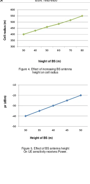
[image:6.595.160.435.560.720.2]Figure 4. Effect of increasing BS antenna height on cell radius
Figure 5. Effect of BS antenna height On UE sensitivity receives Power.
300 350 400 450 500 550 600
30 40 50 60 70 80
Cell radius
(m)
hieght of BS (m)
‐50
‐40
‐30
‐20
‐10
30 35 40 45 50
pr (dBm)
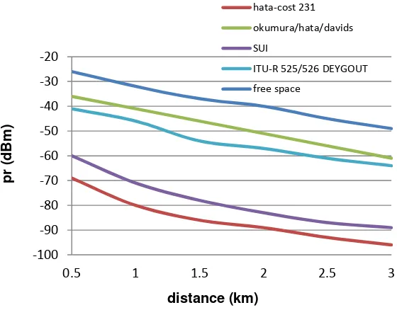
Figure 6. Comparison of different propagation models in UTM
In practice, different clutters will be experienced along a particular path at a given distance, due to multipath effects. In the proposed simulation coverage scheme, each color represents different signal strength. For example, light brown color shows the area with the maximum signal strength, light blue color represents the area with minimum signal strength; while dark blue color represents the area without signal coverage. Assuming that a carrier frequency of 2.6 GHz and less than 10 BTS were used for UTM area, it was observed that the coverage will be too poor and also some areas will not be covered. This is because the frequency is high and therefore cannot penetrate the building walls and thick forests. The received signal strength degrades with increasing propagation loss over cell radius, as shown in Figure 3. The interference from cell center to cell edges is considered is also put into consideration. Increased interference was observed at cell edge, thereby contributing to reduced signal-to-noise ratio (SNR) at the cell boundaries.
The relationship between received signal strength at the user over two-way mode (UL & DL) and cell radius has also been illustrated Figure 3, based on the link budget shown in Table 2. In order to improve coverage distribution, the DL and UP performances must be taken into account. It should be noted that DL and UL transmissions are asymmetrical in terms of maximum transmit power, according to the transmitter characteristics (BS or users’ equipment UE). The effect of cell radius on signal strength is shown in Figure 3. The received signal strengths are -107 and -123.4 dBm in the cell boundaries at the user and from the user at BS respectively. The BS sensitivity is much higher compared to UE sensitivity; and therefore this signal is enough for processing in the BS.The effect of BS antenna height on cell radius for UTM is shown in Figure 4. The cell radius increased from 400 to 560 m, by increasing the height from 30 to 80 m. The UE sensitivity receive power is also increased by increasing BS antenna height, as shown in Figure 5. Figure 6 is a comparison of performances of different radio propagation models used for LTE (such as free space, Okumura/Hata/David’s, Stanford University Interim (SUI), Hata COST-231, and ITU-R 525/526 DEYOUT). It is observed that the Okumura/Hata/David’s model shows the lowest path loss; which implies the highest receive power sensitivity, about (-61 dBm) from the distance (3 km). In contrast, the COST 231 Hata model shows the highest path loss in urban area, implying the weakest receive power sensitivity, about (-96 dBm) from the same distance.
‐100
‐90
‐80
‐70
‐60
‐50
‐40
‐30
‐20
0.5 1 1.5 2 2.5 3
pr (dBm)
distance (km)
hata‐cost 231
okumura/hata/davids
SUI
ITU‐R 525/526 DEYGOUT
5 Conclusions and Future Work
Among the multiple emerging technologies, LTE is a well positioned candidate to meet the requirements of 4G mobile network for both users and operators. LTE is designed to provide greatly improved user experience; and the technology has solved a large number of technical issues faced by the previous mobile communication systems. LTE dimensioning is considered as the main stage in the radio planning process. This paper has presented detailed LTE dimensioning by using ATDI ICS TELECOM. The effects of all parameters (BS height, number of transmitting antennas, region capacity nature, user equipment sensitivity, and so on) on the LTE system performance have been discussed. The performance evaluation of LTE cellular network has been simulated and evaluated in terms of network coverage. The comparison of different propagation models with the proposed model for UTM has also been presented.
Future Work: LTE network planning for coverage and capacity can be implemented by using an alternative tool, such as atoll. The software (atoll) is a 64-bit multi-technology software and has automatic network parameter optimizations for increasing the radio network coverage and capacity.
References
[1] Astély, D., et al. LTE: the evolution of mobile broadband. Communications Magazine, IEEE. 2009;
47(4): 44-51.
[2] Bahattin, K., A. Hüseyin, and Ç. Hakan A. An adaptive channel interpolator based on Kalman filter for
LTE uplink in high Doppler spread environments. EURASIP Journal on Wireless Communications and
Networking. 2009.
[3] Mathew, S. LTE Performance Measurement In Trial Network & Validation Of LTE Performance
Estimation Models. 2012.
[4] Kottkamp, M. LTE Advanced Technology Introduction. White paper, Rohde & Schwarz. 2010.
[5] Kiiski, M. LTE-Advanced: The mainstream in mobile broadband evolution. Wireless Conference (EW),
2010 European. IEEE. 2010.
[6] Abed Astély, D., et al. LTE: the evolution of mobile broadband. Communications Magazine, IEEE.
2009; 47(4): 44-51. G.A., M. Ismail, and K. Jumari. The Evolution to 4G Cellular Systems: Architecture
and Key Features of LTE-Advanced Networks. Spectrum. 2012; 2(1).
[7] Holma, H. and A. Toskala. LTE for UMTS-OFDMA and SC-FDMA based radio access: Wiley. 2009.
[8] Sesia, S., I. Toufik, and M. Baker. LTE–The UMTS Long Term Evolution. From Theory to Practice,
published in. 2009: 66.
[9] Motorola, L.T.E. A technical overview. Technical White Paper. 2007.
[10] Rumney, M. Introducing LTE Advanced. Agilent Technologies. 2011: 22.
[11] Aldhaibani, J.A., et al. On Coverage Analysis for LTE-A Cellular Networks. International Journal of
Engineering and Technology. 2013.
[12] Hussein, N.M., et al. LTE Network Dimensioning Tool Using Java. International Journal of Advanced
Research in Electronics and Communication Engineering. 2012; 1(3): 1-10.
[13] Zhang, L. Network Capacity, Coverage Estimation and Frequency Planning of 3GPP Long Term
Evolution. Linköping. 2010.
[14] Ahmad, Y.A., W.A. Hassan, and T. Abdul Rahman. Studying different propagation models for LTE-A
system. Computer and Communication Engineering (ICCCE), 2012 International Conference on. IEEE. 2012.
[15] Shabbir, N., et al. Comparison of Radio Propagation Models for Long Term Evolution (LTE) Network.
arXiv preprint arXiv:1110.1519. 2011.
[16] Rani, M.S., et al. Comparison of Standard Propagation Model (SPM) and Stanford University Interim
(SUI) Radio Propagation Models for Long Term Evolution (LTE). 2012.
[17] Klozar, L. and J. Prokopec. Propagation path loss models for mobile communication. Radioelektronika
(RADIOELEKTRONIKA), 2011 21st International Conference. IEEE. 2011.
[18] Sharma, P.K. and R. Singh. Comparative analysis of propagation path loss models with field
measured data. International Journal of Engineering Science and Technology. 2010; 2(6): 2008-2013.
[19] Podder, P.K., et al. An Analytical study for the performance analysis of propagation models in WiMAX.
International Journal Of Computational Engineering Research. 2012; 2: 175-181.
[20] Farooq, E.M., E.M.I. Ahmed, and E.U.M. Al. Future Generations of Mobile Communication Networks.
[21] Holma, H. and A. Toskala. Wcdma for Umts. Citeseer. 2000; 4.
[22] Patil, C., R. Karhe, and M. Aher. Development of Mobile Technology: A Survey. Development. 2012;
1(5).
[23] Prajesh, P. and R. Singh. Comparative mesurement of outdoor propagation pathloss models in BHUJ,
[24] Nubarrón, J. Evolution Of Mobile Technology: A Brief History of 1G, 2G, 3G and 4G Mobile Phones.http://www.brighthub.com, 2011.
[25] Armoogum, V., et al. Comparative study of path loss using existing models for digital television
broadcasting for summer season in the north of mauritius. Telecommunications, 2007. AICT 2007. The Third Advanced International Conference on. IEEE. 2007.
[26] Shahajahan, M. and A.A. Hes-Shafi. Analysis of propagation models for WiMAX at 3.5 GHz. MS
thesis. Blekinge Institute of Technology, Karlskrona, Sweden. 2009.
[27] Abhayawardhana, V., et al. Comparison of empirical propagation path loss models for fixed wireless
![Table 1. Values of constantsa, b and cUsed for terrains [22]](https://thumb-ap.123doks.com/thumbv2/123dok/248047.503947/3.595.127.472.220.261/table-values-constantsa-b-cused-terrains.webp)
![Table. 2 Uplink and Downlink Budget parameters[7]](https://thumb-ap.123doks.com/thumbv2/123dok/248047.503947/5.595.136.459.260.433/table-uplink-and-downlink-budget-parameters.webp)