DOI: 10.12928/TELKOMNIKA.v14i4.3985 1438
Novel DV-hop Method Based on Krill Swarm Algorithm
Used for Wireless Sensor Network Localization
Yang Sun1, Shoulin Yin*2, Jie Liu3
Software College, Shenyang Normal University, Shenyang, China No.253, HuangHe Bei Street, HuangGu District, Shenyang, P.C 110034 - China
*Corresponding author, email: [email protected], [email protected], [email protected]
Abstract
Wireless sensor network (WSN) is self-organizing network; it consists of a large number of sensor nodes with perception, calculation ability and communication ability. Generally, the floor, walls or people moving has an effect on indoor localization, so it will result in multi-path phenomena and decrease signal strength; also the received signal strength indicator (RSSI) is unable to gain higher accuracy of positioning. In order to improve the WSN positioning accuracy in indoor condition, in this paper, we firstly propose krill swarm algorithm used for WSN localization. We detailed analyze the multilateral measurement method in range-free distance vector-hop (DV-hop) localization algorithm. The position problem can be transformed into a global optimization problem. Then, we adequately utilize the advantage of calculating optimization problem and apply the krill swarm algorithm into the stage of estimating unknown node coordinates in DV-hop algorithm to realize localization. Finally, the simulation experience results show that the localization with krill swarm algorithm has an obviously higher positioning precision and accuracy stability with different anchor node proportion and nodes.
Keywords: WSN, RSSI, DV-hop localization algorithm, krill swarm algorithm, range-free distance,
multilateral measurement method
Copyright © 2016 Universitas Ahmad Dahlan. All rights reserved.
1. Introduction.
Recently, people have a growing demand for indoor location information services. The traditional GPS and cellular network positioning technology cannot meet the requirements of indoor positioning. Fortunately, wireless sensor network (WSN) [1] makes up for the deficiencies of the traditional positioning technology, which is widely used in exhibition center, intelligent building, sports venues and other fields. In indoor positioning technologies, the localization algorithm performance is directly related to the location accuracy of sensor network node. Currently, WSN localization technology has two major methods: range distance and range-free distance. It includes convex programming localization algorithm [2], centroid localization algorithm and DV-hop localization algorithm [3] based on the range-free distance in WSN node localization. These algorithms work without additional hardware support and high cost. The positioning precision, however, cannot meet the requirements of indoor localization accuracy. The range distance localization algorithms contains time of arrival (TOA) algorithm [4], receive signal strength indication (RSSI) algorithm and angle of arrival (AOA) algorithm. Moreover, some newest machine learning algorithms have been proposed such as [5-7]. In this paper, we design a new method based on Krill Swarm algorithm used for wireless sensor network localization. What’s more, we also state its working principle and demonstrate the indoor localization performance through rigorous experiments. The rest of this paper is organized as follows: The next section of the paper introduces the general principles of the Krill Swarm algorithm and DV-hop algorithm. Section3 proposes the Krill Swarm algorithm used for the WSN localization. After that, experimental results with the Krill Swarm algorithm are presented in section 4. The final section of the paper includes the concluding remarks.
2. Novel DV-hop Method Based on Krill Swarm Algorithm
process of multi-objective, which is very closely to sensor nodes. The aim of our new method is to add sensor nodes density and approach to main node. Using krill swarm algorithm will make each node change their position frequently toward the optimal value direction moderately. Position changing and foraging behavior caused by other anchor nodes contain a local search strategy and a global search strategy. Two kinds of strategies work in parallel. After collecting the optimal position of nodes based on krill swarm algorithm, then we utilize DV-hop method to calculate the position of unknown nodes. Finally, we demonstrate its high performance and efficiency through many experiences. The anchor nodes model with krill swarm algorithm is as follows:
1. Determine the anchor nodes Lagrangian model based on krill swarm.
i i i
i N F D
dt
dX
(1)
Where i is i-th anchor node. Xi is the state of anchor node. Ni denotes velocity vector of
induced movement. Fi is velocity vector of finding key node. Di is random diffusion velocity
vector.
2. Motion induced by other anchor node individuals.
old t n et t i local i new
i
N
N
N
min(
arg)
(2)
Where Nmin=0.1m/s is the minimum velocity of induced movement in WSN based on the real
situation .
n
(
0
,
1
)
is the inertia weight of induced movement. old iN
is the last velocity
vector of induced movement.
local i
is local influence of adjacent anchor node.
NN j j i j i locali K X
1 , , ˆ ˆ (3) best worst j i j i K K K K K , ˆ (4) || || ˆ , i j j i j i X X X X X (5)
Where Ki denotes fitness of i-th anchor node. Kj is fitness of j-th neighborhood anchor node.
Kbest and Kworst are the best fitness and the worst fitness respectively. Xi is the state of i-th
anchor node. Xj is the state of j-th anchor node.İ is a small positive number to avoid
singularity. NN is the number of adjacent anchor node, which can determined by perception
distance of each anchor node di. di can be expressed as:
N j j ii X X
N d 1 || || 5 1 (6)
Where N is the total number of anchor node.
et t i
arg
is influence of the optimal anchor node as (7)best i best i et t
i K X
I
rand , ,
max
arg ˆ ˆ
) 1 ( 2 (7)
Where rand is random number between 0 and 1. I is the current iterations number. Imax is the
3. Finding key node. old i f best i food i f new
i V F
F (
)
(8)
Where
Vf=0.2m/s is speed of finding key node.
f
(
0
,
1
)
is the inertia weight of finding keynode.
ibest is the best previously visited position of the i-th anchor node individual.F
iold isthe last velocity vector of finding key node.
ifood is influence of i-th anchor node, which can be represented by:
N j i N i i ifood X K K
X 1 1 / 1 / (9) food i food i food
i K X
I I , , max ˆ ˆ ) 1 ( 2
(10)So the influence of current i-th node is:
ibest i ibest i best
i Kˆ , Xˆ ,
(11)
This is the finding key node stage. 4. Stochastic diffusion process.
) 1 ( max max I I D
Dinew
(12)
Where Dmax
(0.002,0.01)m/s is the speed of random diffusion. į is the direction vector,which is subjected to (-1,1) uniform distribution. 5. Updating anchor node positions.
)
(
1 new i new i new i I i Ii
X
t
N
F
D
X
(13)
Where
t
is interval selected according to the real situation. In this paper,
t
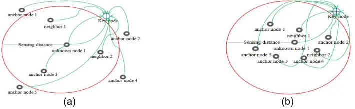
=1s. So every anchor node will get the optimal position in the WSN including the unknown nodes. We can use the following figure to show the anchor nodes movement track.(a) (b)
Figure 1. This figure shows the position of anchor nodes in WSN before and after using krill swarm algorithm. (a) Position of anchor nodes without krill swarm algorithm; (b) Position of
2.1. Process of novel DV-hop based on krill swarm. We design the novel DV-hop algorithm as follows:
Anchor nodes average jump distance computation formula is:
i j hop i j jj ii jj iihopi
x
x
y
y
S
ijS
(
)
2(
)
2/
(14)Where i
hop
S
is corresponding average jump distance of anchor node i. j is other anchor nodenumber in anchor node i data table. ij
hop
S
is the hop count between i and j. (xii, yii) and (xjj,yjj) isthe coordinate of
X
iI,X
Ij (the obtained best position by krill swarm) respectively. Therefore,the i
hop
S
is also the optimal corresponding average jump distance. According to the recorded hop information, unknown nodes will calculate the distance from itself to anchor node after receiving average jump distance by formula (15).i hop
i
S
h
d
(15)After calculating the distance, DV-hop algorithm solves the coordinate of unknown nodes by multilateral measurement method.
Known U11(x11,y11), U22(x22,y22), …, Unn(xnn,ynn) and the unknown node K(x,y) when
there are n(n≥3) nodes. d11, d22, …, dnn are the distance from U11, U22,…, Unn to K respectively.
So: 2 2 2 2 11 2 11 2
11
)
(
)
,
,
(
)
(
)
(
x
x
y
y
d
x
x
nn
y
y
nn
d
nn (16)It can be expressed by system of linear equations AL=B, L=(x,y)T,
A
[(
2
(
x
11
x
nn)
2
(
y
11
y
nn)),
,
(
2
(
x
n1|n1
x
nn)
2
(
y
n1|n1
y
nn))]
T (17) T nn n n nn n n nn nn
x
y
y
d
d
x
B
(
21| 1
2
21| 1
2
21| 1
2)
(18)
Because of the range error, environment factors and communication, AL=B can be rewritten as AL+ε=B. İ denotes the energy consumption parameter in WSN. We can get least-square solutions of equations by standard least least-squares method: L=(ATA)-1ATB. dn is measuring
distance with error included in the B. So the calculation result is limited by dn. If the error of dn is
small enough, L can meet the requirements. However, if the error of dn is big enough, the error
of result is big too. Although this method simplifies the process of solving nonlinear equations, it may reduce accuracy of solution. Aiming at this situation, this paper transforms the problem into global optimization.
Assuming that fn is the measurement error between unknown node and anchor
node, so
f
n
(
x
x
nn)
2
(
y
y
nn)
2
d
n.Then the unknown node K(x,y) can be solved.
n i i iiii
y
y
d
x
x
y
x
f
1 2 2)
)
(
)
(
(
)
,
(
(19)When f(x,y) is the minimum value, the total error is very small and (x,y) is the most approach to the real value, so the (x,y) is optical value. Solution of f(x,y) is not limited to an equation, namely although range error of some anchor nodes is big, it has little effect on the solution of (x,y).
algorithm is a better and newest method to solve global optimization problem. Experiment results show that krill swarm algorithm is a better scheme used for WSN localization.
2.2. Detailed DV-hop Algorithm Based on Krill Swarm
Step 1: Initialization. Set the generation counter Q=1; initialize the population P of NP anchor nodes randomly and each node corresponds to a potential solution to the given problem; set the finding key node speed Vf, the minimum diffusion
speed Dmin, and the maximum induced speed Nmax.
Step 2: Fitness evaluation. Evaluate each anchor node according to its position. Step 3: While the termination criteria is not satisfied or Q<MaxGeneration do. Sort the population of nodes from best to worst.
for =1: NP do
Perform the following motion calculation.
Motion induced by the presence of other nodes. Finding key node.
Physical diffusion.
Implement the genetic operators.
Update the node individual position in the search space. Evaluate each krill individual according to its position. end for i
Sort the population of node from best to worst and find the current best. Q=Q+1.
Step 4: End while.
Step 5: Get processed anchor node positions. Step 6: DV-hop correction.
If RSSI value > T, hops count=0.5. Otherwise, hops count=1. Step 7: Hops between nodes acquisition.
Step 8: The average hop distance calculation. Step 9: Position to calculate.
Step 10: Finish
3. Simulation Experiments and Analysis.
In this section, we make experiments to verify the performance our algorithm. The experiments of DV-hop algorithm based on krill swarm is made on MATLAB platform. In 100m*100m region, we randomly scatter 200 nodes. The fixed node communication radius is 30m. Changing the number of anchor node from 20 to 55. We also make a comparison to DV-hop and the method (IDV-DV-hop) in reference [8] with our new scheme (KSDV-DV-hop). After experiments, we get the results and average value as Figure 2.
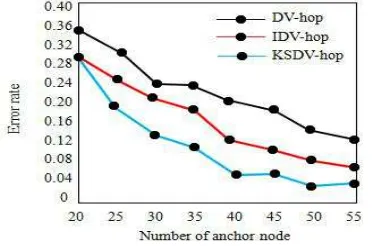
Figure 2. The effect of number of anchor node on error rate
From Figure 2, we can know that this new method is superior to DV-hop algorithm. When the number of anchor node is very small, the error rate decreases rapidly. When the anchor node number is steady, the error rate remains unchanged, which indicates that KSDV-hop algorithm has little requirement for anchor node number. As we all know, anchor node cost with positioning function is far larger than unknown node in WSN, as well as the energy consumption. Therefore, reducing anchor nodes plays an important role in reducing network cost and improving network life cycle. Table 1 is the corresponding data of Figure 3. Keeping the anchor node 50 unchanged, we change the communication radius from 15m to 50m. And it conducts 100 Monte-Carlo simulations as Figure 3.
Table 1. Error rate value with different anchor nodes
Algorithm Number of anchor nodes
20 25 30 35 40 45 50 55 DV-hop 0.361 0.318 0.251 0.262 0.212 0.202 0.168 0.124 IDV-hop 0.301 0.245 0.221 0.197 0.131 0.109 0.105 0.079 KSDV-hop 0.301 0.199 0.146 0.118 0.057 0.061 0.035 0.038
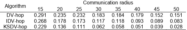
Table 2 is the corresponding data of Figure 4. It shows that Max-Hop of network is decreasing from 15m to 50m. So the position accuracy will improve. The whole of error rate experiences a decreasing trend. On the whole, KSDV-hop algorithm is superior to DV-hop algorithm under any communication radius. Compared to [8], the error rate is very small with our new method. And with proper communication radius, results of KSDV-hop are more stable.
Table 2. Error rate value with different communication radius
Algorithm Communication radius
15 20 25 30 35 40 45 50 DV-hop 0.291 0.235 0.232 0.183 0.184 0.179 0.152 0.151 IDV-hop 0.268 0.178 0.173 0.117 0.118 0.093 0.089 0.083 KSDV-hop 0.229 0.136 0.111 0.062 0.058 0.051 0.039 0.028
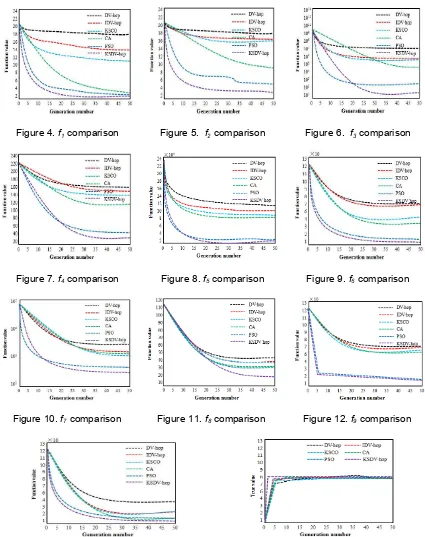
What’s more, we make experiments with 10 standard testing functions (Multimodal functions: Ackley f1, Fletcher-Powel f2, Griewank f3, Penalty f4, Quartic f5, Rastrigin f6; Unimodal
functions: Rosenbrock f7, Schwefel 12 f8, Sphere f9, Step f10) to compare DV-hop, IDV-hop,
KSCO (Krill swarm crossover operator in [9]), CA (cuckoo algorithm [10]), PSO (particle swarm optimization in [11]) to our KSDV-hop method. Supposing that population size NP=50, and maximum generation Maxgen=50 for each algorithm. We ran 100 Monte Carlo simulations of each algorithm on each bench mark function to get representative performances and the results are as table4 including average minima value (amv) and best minima value (bmv).
Table 3. Simulation results
DV-hop IDV-hop KSCO CA PSO KSDV-hop
amv bmv amv bmv amv bmv amv bmv amv bmv amv bmv
f1 4.42 7.64 3.75 5.38 3.52 4.13 2.58 5.84 3.64 5.87 1.42 1.29
f2 6.87 6.59 4.62 3.35 2.38 2.84 3.64 1.62 4.73 7.66 1.23 1.08
f3 32.64 36.12 18.97 18.05 9.65 16.87 11.32 20.85 20.56 22.37 4.26 1.59
f4 2.3e 3
3.2e3 25.63 18.67 18.95 15.66 1.4e4 3.6e4 3.1e3 2.8e3 5.57 3.17
f5 86.34 67.59 52.87 48.67 35.64 35.65 44.83 45.84 96.57 87.34 18.23 9.63
f6 86.34 78.65 75.12 65.34 46.95 45.77 50.28 46.29 87.64 60.85 20.31 1.67
f7 8.87 18.36 6.53 11.78 5.55 6.53 6.13 5.78 7.86 10.46 1.25 1.45
f8 6.95 12.47 5.21 12.31 3.37 5.87 4.29 6.75 5.28 8.87 1.46 1.11
f9 12.64 9.76 10.28 8.76 8.98 6.54 6.51 6.66 13.74 7.85 1.12 1.13
f10 7.87 13.81 3.94 8.57 3.87 5.36 4.62 4.21 9.55 4.45 1.57 1.05
to get best function value as Figure 4-13 for the ten functions. And the position value as Figure 14. Figure 4-13 show that KSDV-hop can get optimization results in a short time with a low generation number. Among the six optimization algorithms, our method performs the best and most effectively when solving the global numerical optimization problems and significantly outperforms the other five approaches.
Figure 4. f1 comparison Figure 5. f2 comparison Figure 6. f3 comparison
Figure 7. f4 comparison Figure 8. f5 comparison Figure 9. f6 comparison
Figure 10. f7 comparison Figure 11. f8 comparison Figure 12. f9 comparison
Figure 13. f10 comparison Figure 14. True value with different algorithms
4. Conclusions
This paper makes an analysis for traditional DV-hop. In that there are many extra factors, such as environment, measurement error etc. So we propose a novel DV-hop based on krill swarm algorithm. This new method can speed up the global convergence rate without losing the strong robustness of the basic DV-hop. From the analysis of the experimental results, it can be concluded that the proposed DV-hop method uses the information in past solutions more efficiently when compared to the other population based optimization algorithms such as IDV-hop, CA, KSCO, PSO. Based on the results, KSDV-hop significantly improves the performance of DV-hop on most multimodal and unimodal problems. In addition, KSDV-hop is simple and easy to implement.
References
[1] Shahrokhzadeh M, Haghighat AT, Mahmoudi F, et al. A Heuristic Method for Wireless Sensor Network Localization. Procedia Computer Science. 2011; 5: 812-819.
[2] K Ren, F Zhuang. Research and improvement of mobile anchor node localization algorithm based on convex programming. Chinese Journal of Sensors and Actuators. 2014; 27(10): 1406-1411.
[3] W Guo, J Wei. Optimization Research of the DV-Hop Localization Algorithm. TELKOMNIKA Indonesian Journal of Electrical Engineering. 2014; 12(4): 2735-2742.
[4] Sathyan T, Hedley M, Humphrey D. A multiple candidate time of arrival algorithm for tracking nodes in multipath environments. Signal Processing. 2012; 92(7): 1611-1623.
[5] Salem O, Guerassimov A, Mehaoua A, et al. Anomaly Detection in Medical Wireless Sensor Networks using SVM and Linear Regression Models. International Journal of E-Health and Medical Communications. 2016; 5(1): 20-45.
[6] Lv T, Gao H, Li X, et al. Space-Time Hierarchical-Graph Based Cooperative Localization in Wireless Sensor Networks. IEEE Transactions on Signal Processing. 2016; 64(2): 322-334.
[7] Pan MS, Lee YH. Fast convergecast for low-duty-cycled multi-channel wireless sensor networks. Ad Hoc Networks. 2016; 40: 1-14.
[8] Qin Shan Zhao, Yu Lan Hu. An improved DV-Hop localisation algorithm. International Journal of Wireless and Mobile Computing. 2016; 10(1).
[9] Gandomi AH, Alavi AH. Krill herd: A new bio-inspired optimization algorithm. Communications in Nonlinear Science & Numerical Simulations. 2012; 17(12): 4831-4845.
[10] Wang G, Guo L, Duan H, et al. A hybrid metaheuristic DE/CS algorithm for UCAV three-dimension path planning. Scientific World Journal. 2012; 2012(9): 2977-2991.