Analysis of variance

(1)

Analysis of variance

Rudolf N. Cardinal, MA PhD MB BChir MD MRCP Academic Clinical Fellow

Department of Psychiatry, University of Cambridge, Addenbrooke’s Hospital, Hills Road, Cambridge CB2 0QQ, UK.

Telephone: +44–(0)7092–340641. Fax: +44–(0)7092–340645. E-mail: rudolf@pobox.com.

[NOTE: home address for pre-publication correspondence is as previously supplied to Wiley & Sons, but that address is not for publication; address for publication is as above.]

For Weiner IB & Craighead WE (editors), The Corsini Encyclopedia of Psychology, John Wiley & Sons

FILES

• Manuscript: (this file; Cardinal_ANOVA_CorsiniEncyclopedia.doc; Word 97 format)

• Figure 1: Cardinal_Figure_1_ANOVA_illustrations.ai (Adobe Illustrator 11 format)

• Figure 2: Cardinal_Figure_2_SS_and_correlated_predictors.ai (Adobe Illustrator 11 format)

KEY WORDS

(2)

OVERVIEW

Analysis of variance (ANOVA) was initially developed by R. A. Fisher, beginning around 1918, and had early applications in agriculture. It is now a dominant and powerful statistical technique used extensively in psychology. In ANOVA, a dependent variable is predicted by a mathematical model comprising one or more predictor variables, which may be categorical (factors) or quantitative and continuous (covariates; regressors). The model’s best prediction is calculated by minimizing the sum of the squared residuals (errors, or deviations from the model’s prediction). Having done this, the proportion of variance in the dependent variable accounted for by each predictor is assessed statistically, testing the null hypotheses that the mean of the dependent variable does not vary with the predictor(s); good predictors account for a large proportion of the variance, compared to unpredicted (error) variance, and poor predictors account for a small proportion. ANOVA allows the effects of predictors to be assessed in isolation, but also allows the assessment of interactions between predictors (effects of one predictor that depend on the values of other predictors).

ASSUMPTIONS

(3)

LOGIC OF ONE-WAY ANOVA

The basic logic of ANOVA is simply illustrated using a single categorical predictor (single-factor or one-way ANOVA). Suppose A is a factor that can take one of k values (representing, for example, k different experimental treatments), and n values of the dependent variable Y have been sampled for each of the conditions A1…Ak (giving nk observations in total). The null hypothesis is that the dependent variable Y has the same mean for each of A1…Ak, i.e. that A has no effect upon the mean of Y. ANOVA calculates a mean square for the predictor (MSA) and an error mean square

(MSerror) and then compares them.

Mean Square For The Predictor

If the null hypothesis is true, then the k samples have been drawn from the same population, and by the Central Limit Theorem, the variance of the k sample means is an estimator of e /n

2

σ , where σe2 is the population (and error) variance, so n times the

variance of the sample means estimates σe2. However, if the null hypothesis is false,

the sample means have come from populations with different means, and n times the

variance of the k sample means will exceed this value. The sum of squared deviations

(abbreviated to sum of squares; SS) of each condition’s mean from the grand mean

(Y ) is calculated for the predictor, summing across all observations (in this example,

2 2

), and divided by the degrees of freedom

(df) for the predictor (in this example, df_A =k−1) to give the mean square (MS) for the predictor (MS_A =SS_A/df_A). If the null hypothesis is true, then the expected value of this number, E(MSA), is the error variance σe2. If the null hypothesis is false, then

the expected mean square will exceed 2

e

σ , as it will contain contributions from the

non-zero effect that A is having on Y.

Mean Square For Error

Whether or not the null hypothesis is true, the sample variances 2 2

1 Ak

A s

s K estimate the corresponding population variances 2₁ 2

k

A

A σ

σ K , and by the homogeneity of variance

assumption, also estimate the error variance σ_e2. An estimate of σ_e2 is therefore

obtainable from the sample variances 2 2

1 Ak

A s

(4)

deviations after the prediction has been made—is calculated (in this example,

) and divided by the error degrees of freedom (in this

example, df_error =df_total−df_A =[nk− − − =1] [k 1] k n[ −1]) to give

error error error SS /

MS = df . Whether the null hypothesis is true or not, E(MS_error)=σ_e2.

The graphical meaning of these SS terms is shown in Figure 1a.

F Test

Comparison of MSA to MSerror thus allows assessment of the null hypothesis. The

ratio F =MS / MS_A _error is assessed using an F test with (dfA, dferror) degrees of

freedom. From the observed value of F, a p value may be calculated (the probability

of obtaining an F this large or greater, given the null hypothesis). In conventional

approaches, a sufficiently large F and small p leads to the rejection of the null

hypothesis.

INTERACTIONS, MAIN EFFECTS, AND SIMPLE EFFECTS

When multiple factors are used in analysis, a key feature of ANOVA is its ability to

test for interactions between factors, meaning effects of one factor that depend on the

value (level) of other factor(s). The terminology will be illustrated in the abstract,

temporarily ignoring important statistical caveats such as homogeneity of variance.

Suppose the maximum speeds of many scrap cars are analysed using two factors: E

(levels: E0 engine broken, E1 engine intact) and F (levels: F0 no fuel, F1 fuel present).

There will be a main effect of Engine: on average, ignoring everything else, E1 cars go

faster than E0 cars. Similarly, there will be a main effect of Fuel: ignoring everything

else, cars go faster with fuel than without. Since speeds will be high in the E1F1

condition and very low otherwise, there will also be an interaction, meaning that the

effect of Engine depends on the level of the Fuel factor, and vice versa (the effect of a

working engine depends on whether there is fuel; the effect of fuel depends on

whether there is a working engine). One can also speak of simple effects: for example,

the simple effect of Fuel at the E1 level is large (fuel makes intact cars go) whereas

the simple effect of Fuel factor at the E0 level is small (fuel makes no difference to

broken cars). Likewise, the Engine factor will have a large simple effect at F1 but a

small simple effect at F0. Main effects may be irrelevant in the presence of an

(5)

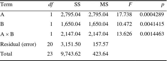
A two-factor ANOVA is illustrated in Figure 1b. ANOVA results are conventionally reported in the form shown in Table 1.

POST-HOC ANALYSIS OF INTERACTIONS AND MULTILEVEL FACTORS Effects of interest in an ANOVA that are found to be significant are frequently analysed further. Interactions may be followed up by analysing their component parts, for example by restricting the analysis to a subset of the data (such as by examining simple effects, or simpler component interactions within a complex interaction). Likewise, significant main effects of interest may require further analysis. For example, if a three-level factor A is found to have an effect, then the null hypothesis

1 2 3 tests is available for this purpose. The most important feature of such tests is that they involve the potential for multiple comparisons, and thus have the potential to inflate the Type I error rate, particularly as the number of levels of the factor increases. Appropriate tests control the maximum Type I error rate for a whole ‘family’ of comparisons.

ANOVA AS A GENERAL LINEAR MODEL (GLM)

More generally, each observed value of Y can be modelled as a sum of predictors each multiplied by a regression coefficient (b), plus error not accounted for by the prediction (e):

In matrix notation, this may be written:

= +

Y Xb e

(6)

of a design matrix allows arbitrary designs including factors with multiple levels, combinations of categorical and continuous predictors, and interactions to be encoded. The matrix b contains coefficients (in this example, b0 is the value of the overall Y

mean, Y ), and e contains errors. This equation may be solved for b so as to minimize the summed squared residuals ( 2

e contribution of any given predictor may be assessed by comparing the predictive

value of a ‘full’ model, containing all predictors, to a ‘reduced’ model containing all

predictors except the one of interest:

(

) (

model[full] model[reduced]

) (

model[full] model[reduced]

)

model[full] model[reduced] error[full]

or, to make clear the equivalence to the logic discussed above,

(

)

predictor predictor predictor

Effect sizes for individual predictors may be calculated in terms of R2 (the

proportion of variance in Y explained) or in terms of b (the change in Y for a given

change in the predictor).

Viewing ANOVA in terms of a GLM makes its relationship to other well-known

analytical techniques clear. For example, ANOVA with a single two-level factor is

equivalent to a two-group t test; ANOVA with a single continuous predictor is

equivalent to linear regression (Figure 1c); and so on. GLMs also subsume techniques

such as analysis of covariance (ANCOVA) and multiple and polynomial regression,

and can be extended to multiple dependent variables (multivariate ANOVA or

MANOVA). General linear models may also be extended to dependent variables with

non-normal (e.g. binomial) distributions via the generalized linear model.

CONTRASTS AND TREND ANALYSIS

GLMs may also be used to perform contrasts to ask specific questions of the data. In

(7)

value of zero under a given null hypothesis. For example, if a factor has 7 levels, one for each day of the week, then the linear contrast

Mon Tue Wed Thu Fri Sat Sun

0.2 0.2 0.2 0.2 0.2 0.5 0.5

L= µ + µ + µ + µ + µ − µ − µ

(where µday indicates the day mean) may be used as a test of the null hypothesis that

the dependent variable is equal on weekdays and weekends. In a GLM, these weights are encoded in a contrast matrix L. After solving Y=Xb+e, the contrast is calculated as L=Lb and assessed statistically to test the null hypothesis L=0.

Trend analysis involves the use of contrasts to ask questions about categorical predictors (factors) that may be treated quantitatively. For example, if subjects’ reaction times are tested with visual stimuli of length 9 cm, 11 cm, 13 cm, and 15 cm, then it may be valid to treat the lengths as categories (do reaction times to the lengths differ?) and quantitatively (is there a linear or quadratic component to the relationship between reaction time and stimulus length?).

CORRELATIONS BETWEEN PREDICTORS AND UNBALANCED DESIGNS When an ANOVA design contains multiple predictors that are uncorrelated, assessment of their effects is relatively easy. However, it may be that predictors are themselves correlated. This may because the predictors are correlated in the real world (for example, if age and blood pressure are used to predict some dependent variable, and blood pressure tends to rise with age). However, it may also occur if there are different sample sizes for different combinations of predictors. For example, if there are two factors, A (levels A1 and A2) and B (levels B1 and B2), then a

balanced design would have the same number of observations of the dependent variable for each of the combinations A1B1, A1B2, A2B1, A2B2. If these numbers are

unequal, the design is unbalanced, and this causes correlation between A and B. This problem also occurs in incomplete factorial designs, in which the dependent variable is not measured for all combinations of factors.

(8)

FIXED AND RANDOM EFFECTS

Up to this point, it has been assumed that factors have been fixed effects, meaning that the levels of the factor exhaust the population of interest and represent all possible values the experimenters would want to generalize their results to analytically; the sampling fraction (number of levels used ÷ number of levels in the population of interest) is 1. A simple example is sex: having studied male and female humans, all possible sexes have been studied. Experimental factors are usually fixed effects. It is also possible to consider random effects, in which the levels in the analysis are only a small, randomly selected sample from an infinite population of possible levels (sampling fraction = 0). For example, if an agronomist wanted to study the effect of fertilizers on wheat growth, it might be impractical to study all known varieties of wheat, so four might be selected at random to be representative of wheat in general. Wheat variety would then represent a random factor.

The most common random effect in psychology is that of subjects. When subjects are selected for an experiment, they are typically selected at random in the expectation that they are representative of a wider population. Thus, in psychology, discussion of fixed and random effects overlaps with consideration of between-subjects and within-subjects designs, discussed below. An ANOVA model incorporating both fixed and random effects is called a mixed-effects model.

With random effects, not only is the dependent variable a random variable as usual, but so is a predictor, and this modifies the analysis. It does not affect the partitioning of SS, but it affects the E(MS) values, and thus the choice of error terms on which F ratios are based. Regardless of the model, testing an effect in an ANOVA requires comparison of the MS for the effect with the MS for an error term where

effect error

(MS ) (MS )

E =E if the effect size is zero, and E(MS_effect)>E(MS_error) if the effect size is non-zero. In fixed-effects models, the error term is the ‘overall’ residual unaccounted for by the full model; in random-effects models, this is not always the case, and sometimes the calculation of an error term is computationally complex.

WITHIN-SUBJECT AND BETWEEN-SUBJECT PREDICTORS, AND MORE COMPLEX DESIGNS

(9)

which each subject is measured at every level of the factor, or a mixture. Within-subjects designs (also known as repeated measures designs) allow considerable power, since an individual at one time is likely to be similar to the same individual at other times, reducing variability. The main disadvantage is the sensitivity of within-subjects designs to order effects.

In a simple within-subjects design, a group of subjects might be measured on three doses of a drug each (within-subjects factor: D). It would be necessary to counterbalance the testing order of the dose to avoid order effects such as improvement due to practice, or decline due to fatigue, or lingering or learned effects of a previous dose. Having done so, then variability between observations may be due to differences between subjects (S), or to differences between observations within one subject; this latter variability may be due to D, or intra-subject error variability (which might also include variability due to subjects’ responding differently to the different doses, written D × S).

For a design involving both between- and within-subjects factors, suppose old subjects and young subjects are tested on three doses of a drug each. Age (A) is a between-subjects factor and dose (D) is a within-subjects factor. In this example, variability between subjects may be due to A, or to differences between subjects within age groups, often written S/A (‘subjects within A’) and thought of as the between-subjects error. Variability of observations within individual subjects may be due to D, or to a D × A interaction, or within-subject error that includes the possibility of subjects responding differently to the different doses (which, since subjects can only be measured within an age group, is written D × S/A). This partitioning of total variability may be accomplished for SS and df and analysed accordingly, with the caveat that as subject (S) represents a random factor, calculation of an appropriate error term may sometimes be complex, as described above.

(10)

an F test as usual but correcting the df to allow for the extent of violation, such as with the Huynh–Feldt or Greenhouse–Geisser corrections; (2) transformation of the data to improve the fit to the assumptions, if this is possible and meaningful; (3) using MANOVA, which does not require sphericity; (4) testing planned contrasts of interest, which have 1 df each and therefore cannot violate the assumption.

(11)

REFERENCES

Cardinal, R. N., & Aitken, M. R. F. (2006). ANOVA for the behavioural sciences researcher. Mahwah, New Jersey: Lawrence Erlbaum Associates.

Fisher, R. A. (1918). The correlation between relatives on the supposition of Mendelian inheritance. Transactions of the Royal Society of Edinburgh, 52, 399–433. Fisher, R. A. (1925). Statistical Methods for Research Workers. Edinburgh: Oliver & Boyd.

Howell, D. C. (2007). Statistical Methods for Psychology, sixth edition. Belmont, California: Thomson/Wadsworth.

Langsrud, Ø. (2003). ANOVA for unbalanced data: use type II instead of type III sums of squares. Statistics and Computing, 13, 163–167.

Maxwell, S. E., & Delaney, H. D. (2003). Designing Experiments and Analyzing Data: A Model Comparison Perspective. Mahwah, New Jersey: Lawrence Erlbaum Associates.

Myers, J. L., & Well, A. D. (2003). Research Design and Statistical Analysis, second edition. Mahwah, New Jersey: Lawrence Erlbaum Associates.

StatSoft (2008). Electronic Statistics Textbook. Tulsa, Oklahoma: StatSoft. URL: http://www.statsoft.com/textbook/stathome.html.

(12)