Simple Model for Simulating Characteristics of River Flow Velocity in Large Scale

Volumr ZOl5,Art1dt ID S20893, 8113g\'S http-J/d.t..dot.orJo'IO. l ISS/lOIS/520893

Research Article

H indawi

Simple Model for Simulating Characteristics of

River Flow Velocity

in

Large Scale

Husin AJatas,

1.2

Dyo D. Prayuda,

1

Achmad Syafiuddin,

1

May Parlindungan,

3

Nurjaman O. Suhendra,

3

and Hidayat Pawitan

1.J

1 _{Re.search Cluster for DynamiCJ and Modeling of Comp/,x Systrms.}

Fac11/1y of Mathematics a11d Natural Scienets. Bogor Agricult1mu Umversity.

JI.

Memnti, KDmpus IPB Darm11ga. Begor 16680, lndones1u

1_{111eoretical Physics Division, Department of PhysiCJ, Bogor Agricultuml University,}

/I. Mtrallti, Kampus IPB Darmaga. Bogor 16680, Indonesia

JH)'drumetturolugy Di11ision, Drpartmtnt of Gtoplrysics and Mrtc:urology. Bugur Agricultural U11i11trsity, /I. Meranti,

Kampw IPB Darmaga, 84'gtJr 16680, lndontsia

Correspondenct should be aJdmsed to Husin Alatas; alatas@ipb.ac.iJ and Hiday.it Pawitan; ｨｰ｡ｷｩｴ｡ｮｾｩｰ｢Ｎ｡｣Ｎｩ､＠ Received 28 July 2014; A.:.:epted 30 Ol!cemb<r 2014

Academic Editor: Alcxey Stovas

Copyright 0 2015 Hus in Alatas d al. This is an open access article distributed under the Creative Commons Attribution License, which permits unrtstrictcd use, distribution, and reproduction in any medium, provided the original work is properly cited.

We propose a simple computer based phenomenological model to simulate the characteristics of river flow velocity in large scale. We use shuttle radar tomography mission based digital ･ｬｾＭ｡ｴｩｯｮ＠ model in grid form to define the terrain of catchment area. The

model relics on mass-momentum conservation law and modified equation of motion of falling body in inclined plane. We asswne inelastic collision occurs at every junction of two nvcr branches to describe the dynamics of merged flow velocity.

1.

Introduction

The complexity of river network has been studied intensively over the past decades in order to describe its pattern forma-tion and dynamics [l

I.

The evolution of river network pattern has been invtsligatcd based on various approaches such as continuum (2-4], stochastic (5], and cellular [6] approaches. On the other hand, one of the most important dynamical characteristics of a river is its flow velocity which corresponds to the water discharge along the river lines. Many different empirical models have been proposed to describe the asso-ciated dynamics in various scales and for various purposes as welJ [7-U). Recently, Gaucl<lcr-Manning-Strickler (GMS) formula based empirical model has been implemented to describe the global river flow in certain area of Europe (9].

In

the meantime, one of the theoretical descriptions of dynamics of open/close river channel is given by the so-called Saint Venant ｾｵ｡ｴｩｯｮｳ＠ (SVEs) in one or two dimensions. These spatiotemporal equations arc developed on the basis of mass-momentum conservation law in the form of coupled continuity and momentum differential equations of average

water discharge and cross-sectional river flow channel func-tio ns where both need initial and boundary condifunc-tions (7,

13-19). Recently, one-dimensional SVE has been adopted in a coupled hydrodynamic analysis model to investigate the large scale water discharge dynamics at basin of Yangtu River.

China, in the presence of complex river-Jake interaction (7).

2 International Journal of Geophysics

s

)3-4 339 3-41 345 JSJ 3S4

34S

m

JS7

343 )4) 348 356

34S 347

2 348

3-411 )Sil )Sil

350 362 36) l66 366

351 353 36? 364 367 370

350 353 357 360 365 365 367 372

3 344 347 351 359 367 3'9 Jn

( a) (b)

FtGUltE I: (a) The network pattern of Ciliwung River catchment ;uea which is divided into five regions. The solid dot rtprtsmls the position of Katulampa obmvation point. (b) Modified DEM data of!JO >< ｾ＠ m! grid resolurion of a smaU arn around Katulampa.

In this report, we propose a simple approach to develop a computer based discrete phenomenological model of river flow velocity. We still rely on mass-momentum conservation law by assuming that an inelastic collision occurs at a river junction. Instead of using GMS formula, to accommodate friction, roughness, and number of rocks in single

param-eter,

here we introduce the notion of effective gravitational

acceleration, whereas the flow velocity follows the equation of motion of falling body in inclined plane.

The procedure that we followed to develop the model includes the following: {i) determination of river catchment area in the form of a computational window grid, (ii)

development of algorithm for flow velocity model, and (iii) examining the model characteristics with respect to the variations of initial water discharges at headwaters.

To our best knowledge, the proposed model has never been reported elsewhere. We compare our model with field observation data in order to justify the results. It should ｾ＠

emphasized from the beginning that this simple model is an attempt to determine characteristics of river flow velocity and it is not intended to replace SVEs. In principle, however, this model can also provide initial condition of the whole river network which is needed to solve numerically the corresponding time -dependent SVEs.

Wt considertd tht catchment :irca of Ciliwung River (CR)

situated in West Java Province, Indonesia. for simulating the model To define the corresponding terrain we used digital elevation model (DEM) in grid form which is constructed based on free shuttle radar topography mission (SRTM) data provided by USGS (20). Each grid in DEM represents the average height within the corresponding terrain. We onJytake into account the surface runoff and exclude the subsurface runoff as well as landscape characteristics of surrounding river lines such as forest canopy. vegetation, land use, and sediment transport.

We organize this report as follows: in Section 2 we discuss the associated DEM of CR catchment area and then this is followed by the explanation of flow velocity model in Section 3. The results of our simulation and its discussion are given in Section 4. We conclude our report by a summary in

Section 5. Sections 2- 4 discuss consecutively the abovemen-tioned procedure that we followed.

2.

DEM of Ciliwung Rivtr Catchment Area

The CR is one of the most important rivers in Java Island, Indonesia. It spans over 120 km from Mount Pangrango in West Java to Java Sea, north to the capital city.Jakarta. Its catchment area is 149 km1. In recent years, during the rainy season, this river contributes around 30% of flood in

Jakarta.

To plot the CR catchment area we used DEM with 90 x 90 m1 grid resolution and in order to get a more detailed terrain which still can be handled by modest computational facility, the associated DEM was corrected by IS x 1 S m2 resolution

DEM

as well

as

data from field survey. Using

GIS

software this modified DEM was converted into numbers that can ｾ＠ read by Excel software. Shown in Figure l(a) is the plot of 90 x 90 m2 DEM of the corresponding CR river network pattern. It is obvious that water will flow to the lower land due to gravitational force, such that we can use this fact

as

a rule in our computer code to determine the corresponding river pattern based on the given DEM data after identifying the positions of all headwaters. There-fore, it is clear that the boundaries of all river branches which define a two-dimensional computational window are automatically provided by DEM, where each grid• represents the corresponding computational mesh. In Figure l(b) we give an example of specific small area of the corresponding computational window grid (sec figure caption) which is highlighted with grey color grid. The number inside each grid represents DEM value in meter unit at specific position.

Based on our modified DEM, we identified that there are 126 headwaters. According to StrahJer classification of river branches, all these headwaters converge into order 4 river channel at Katulampa area with channel dimension of

3. Flow Velocity Model

We consider a discrete model where the water discharge is represented by the corresponding two-dimensional grid in the modified DEM in which its position is denoted b)'

indices (i, j). After determining the river network pattern. we

model the corresponding flow velocity by assuming that its magnitude at particuJar position of water discharge along a river channel is given b)' the following equation:

v(i,

j)

=

ｾｹＮ＠

(i',

j') +

29ttr

(i',

j';

h)

llH, (I)

where v(i',

j')

and v(i, j) dt:note the flow velocity of water

discharge at higher and lower positions, respectively, while 6H

=

H(t.

j') -

H(i, j)

>

O is the height (H) difference,

where the value of H is provided by DEM. The symbol 9.tr

represents the effective gravitational acceleration which is defined to ac,ommodate the real condition of river channels

and h denotes waterlevel from river bed at the position (i'

.j').

Flow velocities in (l) can be interpreted as the average of

velocity in the associated grid. In the meantime, the width and water level of each river branch are assumed to be uniform.

In general, we assume that the parameter 9.tf depends on

position and water level which can be determined empirically through field observation at particular time. The assumption of water level dependency is taken to accommodate the fact

that water flow is more efficient

as

water level increases. But

for the sake of simplicity, here we assume that 9df is uniform

along all river channels and it will be determined later numerically. Comparing with the flow velocity expression in GMS formula, this parameter plays similar role with the ratio

RW

/n

where RH is hydraulic radius of a rivi:r channel and

n

represents roughness coefficient [9].

Next, to model the merging of flows from two dif-ferent branches at a river junction we assume that the collision of water at each junction is inelastic satisfying the mass-momentum conservation law in the following discrete numerical scheme:

Q,

(i,j)

=

Q,

(i,J)

+

02

(i,j} .

p3

(i,j)

=

p,

(i,j)

+Pi

(i.j).

(2)

(3) Here. Q_1, Q_{2 ,} Q₃ and

p

_1,

p

_{2 ,}

p

₃ are the water discharge and

momentum, respectively, as illustrated in Figure 2. Consider

p

=

pQvllt and

Q

= hwv, where h and w denote the water level from river bed and width of the river channel,

respectively, while

v

and v are, respectively, the flow velocity

vector and its magnitude at the corresponding position.

Here, we assume that the channel cross-section (w x h)

is rectangular. Based on assumption that the collision is

inelastic we can find from (1) and (2) the expression of flow

velocity v3 as follows:

1i:wfv1

+ ｨｾｾｶｾ＠ + ｨ

Ｑ

ｨ

Ｒ

ｷ

Ｑ

ｷ

Ｒ

ｾｾ＠

cos8

h

₁w_1v1

+ h

₂w_2v2

(4)

where 8 is the angle between

v

₁ and

v

_2• Note that after

col-lision we only consider the related flow velocity magnitude,

7

F1cuu 2: JUustration of the inelastic collision of two rivtr branchrs.

while its direction follows the shape of the river channel. To ensure that the collision is inelastic. it is important to

emphasize that our 'omputer code

is

set to

run

the water

discharge with slower velocity first, which will be collided by the faste r one.

It is worth to note that this junction model in principle

can be extended to indude more than two merging branches, namely. by adding another discharge and momentum terms

on the left hand side of (2) and (3), respectively. Furthermore.

this model

can

also be modified to accommodate the river

branch bifurcation cases.

An example of a more complicated junction model has

been proposed previously in (21). In that model, flow from

different river channel does not experience inelastic collision. Instead, by defining control volume to each channel, the water from both channels is assumed to flow side by side in the subsequent channel, where the momentum change

of each flow is determined by hydrostatic pressure and

pressure that related to the change or its control volume

as well .;lS interfacial shear force between them. Another

junction model is given in [22) which also considers the application of continuity and mass-momentum conservation law incorporated with momentum and energy correction parameters. The implementations of these models are likely not easy in large scale cases and local boundary conditions arc needed. Comparing with these two models. it is clear that our junction model is far simpler in its implementation, but it is probably less accurate indeed.

In addition, we also assume that after collision the width

w₃ and water le\'el h₃ will change according to the following

chosen relations:

(5)

for

w

1(2) > w2

u>

and

h3 = h,(2) exp

Ｈｐｾ［ＺＺＩ＠

(6)

for h₁

(2j

> h_{201 .} The symbols

a

and

P

are small and

dimensionless real parameters. These assumptions arc taken to model the width and water level of river channel that resulted from the merging of two different branches. We consider the width and water level as two independent parameters since both are naturally predetermined. Here,

4

bt determined numerically. In general, however, one might consider that their values should not be the same for different junction and can be determined empirically. Indeed, one 'an choose another type of relation to model the width w> and water level

h>.

However, based on our numericaJ experiment which will bt presented in the next section. the relations given by (S) and (6) so far are the most applicable ones to meet the corresponding river parameters and certainly this assumption must be further clarified by field observation whkh is beyond the scope of this report.

To this end, it is well known that based on the following definition of Froude number for a channt?I with rectangular cross-section

v F r = - - ,

..Jg

x

h (7)

where

9

is the actuaJ gravitationaJ acceleration, one can classify the flow regimes into subcritical (Fr < I), critical (Fr

=

1), and supercritical (Fr

>

l) flow (23). It will

be discussed on the next section that the model seems to accommodate only the case of subcritical flow.

4. Results of Model Simulation and Discussion

To simulate our model, we use the water discharge data sample found from our field surveys during dry season in August, 2013. ｂｾ､＠ on those data samples we consider dividing the 126 headwaters into five regions and choose KatuJarnpa as the simulation point as shown in Figure l(b). The corresponding data of headwaters and Katularnpa point were considered as the associated initial and finaJ conditions. respectively.

The initial flow velocity, width, and wate.r level from field survey in each region are assumed to be uniform as given in Table 1. Prior to discussing the characteristics of

our

model

with respect to the initiaJ flow velocity and water

level variations, we first simulate the flow velocity, water level, and width at Katul:unpa with initial values given in Table 1. Our simulation yields the following results: v

=

0.94

mis,

h = 0.41

m,

and w = 70.01 m. On the other hand, from field survey, we observed the following data: 1• ::: 0.90

mis,

h ::: 0.S m, and

w

:::

60.63 m. To meet the simulation results that match Katulampa data, we adjusted by trial and error the parameters in (1), (5), and (6) and found the following vaJues:

9,tr

=

9xlo-s m/s1,a

=

6.3x 10-1,andp

=

s.sx10-1_{, whereas}

in our computer code we run the initial water discharge from region I first and then from regions 2, 3, 4, and 5, respectively, since v0•1

<

v0.i < vo.J < v0 •4 < vo.s· It is worth to note that by assuming

g

-

9.81 m/s1 all these velocities at headwaters and Katulampa are related to subcriticaJ flows according to Froude number given by (7).

The simulation results of flow velocity, water level, and width of the whole catchment area of CR are given in Figure 3. Comparing to our data sample. the simulated flow velocity width and water level do not represent most of the actuaJ conditions although at KatuJampa these quantities are in good agreement This can be explained as a consequence of not applying actual data of the whole headwaters to our

International Journal of Geophysics

TABLE I: Initial lluw vdocity (vu). width (w.,). and water level (ho) of tach chosen rtgson .

ｒ｣ｾｩｯｮ＠ v0 (mis) w0 (m) l1o (m)

I 0 .342 4.85 0.20

2 0.429 3.12 0.10

) _{0.437 1.81 0.30}

4 0.527 1.55 0.30

5 0.940 2.77 0.40

model. One might expect that the use of actual data of all headwaters and considering position-dependent 9dl•

a,

and

fJ will give fairly accurate results with tolerable deviations.

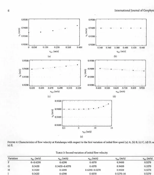
As shown in Figure 3(a), it is found that at every river branch junction, the flow velocity of merged water discharge is getting slower due to inelastic collision given by (3), which corresponds to kinetic energy losses phenomenon.

Next, to simulate the characteristics of flow velocity at Katulampa, we vary the initial flow velocity at headwater of particular region while keeping the velocity of other regions the same. Given in Table 2 are five different variations of the first one, denoted by letters A, 8, C, 0, and

E.

with the co rresponding results depicted in Figure 4. In variation A,

we vary the initial flow velocity v_0•1

=

0-0.4290 mis. It is found that the flow velocity at Katulampa exhibits nonlinear variation as shown in Figure 4(a). However, it should bt noted that the change is relatively small. In contrast, as shown in Figure 4(b), we observe for variation

B,

where

vcu

=

0.3420-0.4290

mis

variation is considered, that the flow velocity at KatuJampa does not

vary

at all. On the other hand, the other different characteristics are found for variations

C

and

D,

with the corresponding variations givt'n a5 follows: v0.l = 0.4290-0.S270m/s and v0.4 = 0.4370-0.9400 mis, respectively. As shown in Figures 4(c) and 4(d), both variations exhibit opposite characteristics, where in variation C the flow velocity is increasing ｡ｬｭｯｾＱ＠ linearly, while for variation D the flow velocity is decreasing linearly. Io the meantime, the variation E given in Figure 4(e) is sin1ilar to variation A where its variation is nonlinear with respect to the lint'ar variation of initial flow velocity v_0,5 =

0.5270-l 4 mis.

For comparison, we also consider another five variations of the second one, denoted by letters F, G, H, I. and

J,

with the corresponding variations of initial flow velocity of each region given in Table 3. Here, we exchange the initial flow velocity between region 4 and region 5 such that vo.4

>

vo,s. The results are depicted in Figure 5. Comparing variations

(a)

0.4

0.3

e

0.2 ｾ＠

0. 1

0 (b)

1.4

1.2

o.s

ｾ＠

0.6 0.4 0.2

0

(c )

60

40

-.§.

20

0

FtGVll! 3: Global pattern of (a) flow vdocity, (b) water level, and (c) width. In these figures we set to zero all the corresponding valuts outside the river chan nels.

T.o u 2: First vcriation ofiniti.il flow velocity.

Variation v₀₁₁ (mis) v₂.2 (mis)

A 0 -0.4290 0.4290

B 0.3420 0.3420-0.4370

c

0.3420 0.4290

0 0.3420 0.4290

E 0.3420 0.4290

To complete our investigation on the flow velocity char-acteristics at Katulampa with ｲｾｳｰ･｣ｴ＠ to initial flow velocity variation, we also simulate the model by uniformly increasing the value of initial flow velocity of each region. The results arc given in Figure 6 showing ｮｯｮｬｩｮｾｲ＠ variation of velocity at

Katulampa with respect to the uniform increment of all initial

flow velocities by Av_{0 .}

Clearly, since it is considered that the water levd docs not vary and that the related velocity at Katulampa tends to grow exponentially, then the corresponding Froude number at that point, which is given by (7), can probably be of Fr

»

1.

Therefore, based on this fact it is safe to say that our model most Likely cannot describe the supercritical flow in a fairly accurate way.

All these results obviously indicate that the influence of initial flow velocity variation at headwaters will lead to specific characteristics of flow velocity at lower land. However, the associated characteristics cannot be easily explained due to complex interaction under inelastic collision among the corresponding river branches. This situation can be txemplified

by

the nonlinear characteristic of variation E

v0,> (mis) v014 (mis) ｶｾ＠ (mis)

0.4370 05 270 0.9400

0.4370 05 270 0.9400

0.4290- 05270 0.5270 0.9400

0.4370 0.4370- 0.9400 0.9400

0.4370 0.5270 0.5270-14

which is clearly different compared to variation I with flat characteristic, although both variations have the same initial flow vtlocity variation on the related region (0.5270-14 mis) and the location of the corresponding headwaters is relatively close to Katulampa as shown in Figure I.

We have discussed previously in Section 3 that in general the panmeler 9df depends on water level. Therefore. in addition to the aforementioned variations, we have also investigated the characteristics offlow velocity and water level at Katulampa by increasing linearly the water level of each headwater as follows:

(8)

with

Ah

= 0.1 x

nm,

where

n

is an integer. In the mean· tiint, the effective gravitational acceleration is considered to increase linearly based on the following equation:

6 International Journal of Geophysics

0.9500 0.9500

..

.

-

...

0.9400

•

';>

..s

-

...

0.9400

!

>' 0.9300 t' 0.9300

0.9200 0.9200

0 0.050 0.150 0.250 0.350 0.450 0.3-W 0.)60 0.380 0.400 0.420 0.440

Vu.1 (mJs) v0J (mis)

(a) (b)

0.9500 ＰＮＹｾ＠

ｾ＠ 0.9400

..

.

.

. ｾ＠ 0.9400

...

..

. . ,

.• . ..

· .. .

i

..

!

"

0.9300 t' 0.9300

0.9200 0.9200

0.430 0.450 0.470 0.490 0.510 0.530 0.420 0.520 0.620 0.720 0.820 0.920

v₀J (mis) v0•4 (mis)

(c) (d)

0.9500

..

.

.

-;;;- 0.9400

.... ...

.

·•

....

• .

!

t' 0.9300

0.9200 ..._ _ _ _ ｾＮ｟｟｟＠ _ _ _ ___. _ _ _ _ __,

0.5 5

V<15 (mf5) (e}

[image:6.614.21.537.39.625.2]

JO 15

FIGURE 4: Characteristics of flow velocity at Katulampa with respect to the first variation of initial flow speed (a) A, (b) 8, (c) C, (d) D, and (e) E.

TABLE 3: Second variation of initial flow velodty. Variation v!!.1 (mis) VPi.1 (mis)

F 0-0.4290 0.4290

G 0.3420 0.3420-0.4370

H 0.3420 0.4290

I 0.3420 0.4290

1

0.3420 0.4290

which is taken under the assumption that higher water level will flow more easily. Here

ho

is given in Table l. The result is shown in Figure 7. It is found that the flow velocity variation

at Katulampa increases nonlinearly with tendency of satura-tion while the corresponding water level increases linearly.

Finally, it should be adm itted that our simple model must be further examined by field observation which should be conducted in relatively long time period. However, this model can be used to determine and predict qualitatively the characteristics of river flow velocity in large scale.

In

additjon, for a relatively small grid DEM, in principle, the calculated

ｶＡＡＮｾ＠ (m/s) vu {mis) v₂J (mis)

0.4370 0.9400 0.5270

0.4370 0.9400 0.5270

0.4290-0.5270 0.9400 0.5270

0.4370 0.5270-14 0.5270

0.4370 0.9400 0.4370-0. 9400

velocity, water level, and width can be used as initial condition of time-dependent SVEs.

5.Summary

09500

-;;-

ｯＮｾ＠

";:a

c >' 09300

0.9200 ｾｾ ＭＭＭｾＭＭＭＭＭＭＭＭＭＭＭＧ＠

0

o.oso

0.150 0.250 O.lSO 0.450 Va.I (mis)

(a) 0.9500 ＮＮＮＮＮＮＭＭＭＭＭＭＭＭｾＭＭｾＭＭｾ＠

- 0 .9400

i

ｾ＠ 0.9JOO

.

.

_..

..

. .

.

.

•

..

0.9200 ｾＭＭＭＭＭＭＭＭＭＭＭＭＭＭＭＭ

0.430 0.450 0.470 0.490 O.SIO 0.530 v_{0_,} (mis)

(c)

0.9500

- 0.9400

!

ｾ＠ 0.9300

0 .9500 ＮＭＭＭＭｾＭＭＭＭｾＭＭｾＭＭＭＭＮ＠

- 0.9400

i

ｾ＠ 09300

o.noo .___ _____________

__,

O.'.ISOO

- 09400

!

ｾ＠ 0.9300

0.)40 0.)60 0.380 0.400 0.420 0.44-0

"11.2 (mis)

(b)

. ..

····•

.

.

.

.

.

.

.

0.9200 ＮＮＮＮＭＮＭＭＭＭＭＭＭＭＭｾＭＭＭＭＭＧ＠

o.s 5 10 IS

"o,4 (mis) (d)

.

..•.

.

'

..

0.9200 .__ _ _ _.... _ _ _ _ _ _ _ _ _ _ . . - J

0.420 0.520 0.620 0.720 0.820 U20

vG.$ (mis) (t)

F1GURE S: Characteristics of now velocity at Katulampa with respect to the second variation of initial flow spttd (a) F, (b) G, (c) H, (d) J, and (t)

J.

1.1500

1.1000

I

1.osoo

ｾ＠ 1.0000 0.9500

.

'

ｾ Ｍﾷﾷﾷ Ｎ＠

.. ....

-

...

..

· .. .

0.9000 ._____...._..__ _ _ _ _ _ ｾ＠ _ _ __.... _ _ ___.

0

ｾ＠

ｾ＠

0 0

ｾ＠

0

ｾ＠

0

0 0 0 0

N .,.. N <r

ci c:i 0 ci ci ci 0 ci

0

Av0 (mis)

F1c11u 6: Characttristic of flow velocity at Katubmpa with respect to uniform increasing of io itial flow spctd of all regions.

The flow velocity is described by equation of motion of falling body in inclined plane due to gravitational force.

We define the effective gravitational acceleration parame-ter to a·ccommodate the real condition of river channel. At the junctfon of two river branches we assume that the merged flow velocity is determined by inelastic collision.

It

is found that our model can determine the flow velocity at Katulampa in ｧｾ､＠ agreement with observation data. The variations of initial flow velocity of certain region in the Ciliwung River headwaters show various characteristics that we suspect to occur due to complex interaction among the river branches. This simple model can be used to determine and predict the characteristics of river flow velocity at subcritical level as well as providing an initial condition for time-dependent Saint Venant equations.

Conflict of Interests

8

Ｖｾｾｾｾｾｾｾｾｾｾｾｾｾｾｾｾ＠

s

0 0.2 OA 0.6 0 8 I ? IA I 6 I 8 2 t.l1(m)

(a)

- 3

i

ｾ＠ 2

•

•

lnternation3l Journal of Geophysics

.. .

•

...

.

.

.

..

ﾷｾｾ ｾｾＭＭｾ ｾｾｾｾｾｾＭＭｾｾｾ＠

0 0.2 0.4 0 6 0.8 I 1.2 I 4 1.6 I 8

t.h (m)

(b)

flGUREi 7: (;a) Ch:aracteristics of water level and (b) flow vdocity (dashed cirde) at Katul:unpa with respect to uniform increasing of initial w-.iter level of all ｲｾｯｮｳ Ｎ＠

Acknowledgment

This work W3S funded by

BOPTN

Research Gr3nt of ｹｾ｡ｲ＠

2013 from Directorate of Higher F.duc3tion, Minist ry of National Education and Cultu re, Republic of Indonesia, under Contract no. 198/IT3.41.2/L2/SPK/2013.

Referencn

Ill

W Wu, Computational Rivtr Dynamics, Taylor & Frands, London, UK. 2002.

12) A. Giacometti, A. Maritan, and

J.

R. Banavar, "Continuum model for river networks; Pliysicnl Review Lttttrs, vol. 75. no. 3, pp. 577-580. 1995.

(3) F. Metivier, ·oiffwivelike buffering and saturation of luge rivers; Plrysical Rniiew E: St'1tistiwl Physics. Plasmas, Fluids. and Rtlattd lnttrduciplinary Topics, vol. 60, no. 5, pp. 5827-5832, 1999.

(4) A. Giacometti. ·Local minimal energy Jandscapts in river networks; Plrysical Review E, vol. 62. no. 5, pp. 6042-6051, 2000. (5) G. Yan,

J.

Zhang. H. Wang, and L Guo. ·simple stochastic lattice g;u autom3ton model for formation of river networks; Physical Revitw E. vol 78. no. 6. Article ID 066102. 2008.

(6) G. Caldardl.i, A. Giacometti, A. Maritan, I. Rodriguez-Itu rbe, and A. Rinaldo, ·Randomly pinned landscape evolution,• Phys-ical Rtvitw £-StatistPhys-ical Physics, Plasmas, Fluids, and Related lnttrdisciplinary Topics, vol 55, no. 5, pp. R4865-R4868, 1997. (7) X. Lai. J. Jiang. Q. Uang, and Q. Huang. · 1.arge-scale

hydro-dynamic modeUng of the middle Yangtu River Basin v.itb complu river-lake interactions; Journal of Hydrr>logy. vul. 492, pp. 223-243. 2013.

(8) M. E. Akiner and A. Ak.koyunlu. ·Madding and forteasting river now rate from the Melen watershed, Turkey." Journal of Hydrology, vol. 456-457, pp. 121- 129, 2012.

(9) K. Verzano, I. Birlund, M. Florke et al., ·Modeling variable rh·er now velocity on continental scale: cunent situat.ion and climate change impacts in Europe; Journal of Hydrology, vol 424-425, pp. 238-251, 2012.

(10) G. Steinebach, S. Rademacher, P. Rentrop. and M. Schulz, ·Mechanisms of coupling in river now sin1ulation S)'Stems." /011rnnl of Computational and Applied M'1thematics, vol. 168, no. 1-2. pp. 459-470. 2004.

(11) C. H. 03vid, Z.·L. Yang, and S. Hong. "Regional-scale ri\·er flow modeling using off-the-shdf runoff products, thousands

of mapped rivers and hundreds of ｳｴｾ｡ｭ＠ flow gauges; Envi· ronmtntul Modilling and Softwart, vol. 42, pp. 116-132, 2013. 1121 F. Liu and B. R. Hodges, ·Applying miaopnxessor analysis

methods to river network modelling; Environmental Mudtlll11g

0-Software, vol. 52, pp. 234-252, 2014.

1131 R. Mowsa and C. Bocquillon, ·Approximation z.ones of the Saint-Venant equatioM for flood routing with owrbank tlow; Hydrology and Earth System ｓＮＺｾｮ｣･ｳＮ＠ vol 4, no. 2. pp. 251-261, 2000.

(14) R. Szymkiewkz, "Solution of the innrse problem for the Saint Venant equ;itions; Journal of Hydrology. vol. 147, no. 1-4, pp. 105-120. 1993.

(15) E. ｂｬ｡､ｾＮ＠ M. Gomn-Valentin. J. Dolz.

J.

L ａｲｾｯｮＭｈ･ｲｮ｡ｮ､ｶＺＬ＠

G. Con:stein. and M. 5ancha· Juny, "lnttgr.ition of ID and 20 finite volume ｳ｣ｨ･ｭｾ＠ for computations of water Oow in natural channds." Adwmus i11 Ｂｾｴｵ＠ Ruourct1, \'OI. 42. pp. 17-29, 2012. ( 161 S. K. Ooi, M. P. M. Krutzen, and E. Weyer. ·on physical and data drh·en modelling of irrigation channels; Control Enginttring Prai:tire, vol. 13. no. 4. pp. 461-471, 2005.

(17) V. dos Santos Martins, M. Rodrigue5, and M. Diagne, •A multi-moJd approach to Saint-Venant 4:t1uations: a stability stuJy by LMls." lntmiationnl Journal of Applitd Mathematics und Computer Science, vol. 22, no. 3, pp. 539-550, 2012.

(Ul) T. G. Lkh and L K. Lual, •Boundary conditions for the two-dimensional Saint-Venant equation system,· Applied Mathemat-ical Modtlling, vol. 16, no. 9, pp. 498-502, 1992.

(19) R. Ghostinc. R. Mose, J. Vazquez. A. Ghenaim, and C. Gregoire, ·rwo-dimension3) simulation of subcritical tlow at 3 combining jun'!ion: luxury or necessity?" fr>urnal of Hydraulic Engmttri11g,

vol 136, no. 10, Artido: fD 004010QHY. pp. 799-805, 2010.

(20) http://gdex.cr.usgs.gov/gdex/.

(211 S. Shabayek. P. Steffler. and F. Hicks. "Dynamic model for subcritical combining flows in channel junctions.· Journal of Hydraulic Engineering, vol 128. no. 9, pp. 821-828, 2002.

I

22

I

C. C. Hsu. W.

J.

Ln, and C. H. Chang, "Subcritical open-channel junction flow; Journal of Hydraulic Engi11euing, vol U4, no. 8, pp. 847- 855, 1998.

Scientifica

Hindawi

The Scientific

World Journal