DOI: 10.12928/TELKOMNIKA.v12i4.532 855
Image Deblurring Via an Adaptive Dictionary Learning
Strategy
Lei Li1, Ruiting Zhang2, Jiangmin Kan*3, Wenbin Li4 1,3,4
School of Technology, Beijing Forestry University, 100083, Beijing, China
1 Institute of Atmospheric Physics, Chinese Academy of Sciences, 100029, Beijing, China
2
Canvard College, Beijing Technology and Business University, 101118, Beijing, China *Corresponding author: [email protected]
Abstract
Recently, sparse representation has been applied to image deblurring. The dictionary is the fundamental part of it and the proper selection of dictionary is very important to achieve super performance. The global learned dictionary might achieve inferior performances since it could not mine the specific information such as the texture and edge which is contained in the blurred image. However, it is a computational burden to train a new dictionary for image deblurring which requires the whole image (or most parts)as input; training the dictionary on only a few patches would result in over-fitting. To address the problem, we instead propose an online adaption strategy to transfer the global learned dictionary to a specific image. In our deblurring algorithm, the sparse coefficients, latent image, blur kernel and the dictionary are updated alternatively. And in every step, the global learned dictionary is updated in an online form via sampling only few training patches from the target noisy image. Since our adaptive dictionary exploits the specific information, our deblurring algorithm shows superior performance over otherstate-of-the-art algorithms.
Keywords: sparse representation, adaptive dictionary learning, image deblurring
1. Introduction
Image bluris usually caused by relative motion between the camera andthe scene during the exposure time, e.g., camera shake. Andthis process can be modeled as the following equation:
(1)
Where is the desired sharp image; is the blurred image,that is, the degraded image; is the blur kernel that is assumedto be linearly shift-invariant; is the additive noiseusually assumed as following Gaussian distribution; denotesthe convolution operator. Image deblurring can be seen as aninverse problem of Eq.(1). Given only the degraded image asinput, the goal of blind image deblurring is to inverse the aboveprocess and to recover both and , which are assumed tobe unknown in this case.This is as so-called blind image deblurring which is a fundamental and challenging problem in theimage and signal processing literature [1]-[3]. Image deblurring has many practical applications,such as removing the blur from consumer photographs, computational photography and astronomical imaging.However,it is still an open question to design an efficient deblurringalgorithm.
Traditional approaches to remove image blur are alwaysdone by employing deconvolution method. However, the deconvolution is a severely ill-posed problem, that is,there canbe exponentially many images and kernels that satisfy Eq.(1). To alleviate these issues, many prior assumptionsand regularities are introduced on the structure of and [3]-[9]. The statistical priors of natural images are often utilized. And a commonly used prior on is the heavy-tailed prior [4], that gradients of natural imagesfollow a hyper-Laplacian distribution which was observed byLevin et al..
Recently, using redundant representations and sparse property in nature images has drawn a lot of research attention. Andsparse representation has also been applied in image deblurringand achieved satisfactory performance [7],[10]. Cai et al.proposed a blind motion deblurring method by exploitingthe sparseness of natural images in over-complete
y=xk+n
x y
k n
x k
x k
predefineddictionary (e.g. wavelets, DCT) to help with kernel estimationand sharp image estimation [7]. Jia et al. proposed a newnon-blind image deblurring method which jointly modeledthe sparse representation of natural image patches and sparsegradient priors [11]. Li et al. proposed a blind image deblurring method by combining the sharp and blur dictionary pairand the sparse gradient prior, and estimating the blur kernel,sharp image and sparse coefficients respectively during thedeblurring process [12]. The redundantand over-complete dictionary has been trained on image patches to helpexploit the sparse prior of natural images [7],[11],[12].
Although deblurring with a prespecified dictionary is simpleand fast, it results in low performance in most cases [13]. Thereason is that the generic bases (i.e., pre-defined basis suchas curvelets and framelets) do not exploit rich informationcontained in the blurred image or the global learned dictionarydoes not transfer well to different types of images. In [14],Hu et al. proposed a deblurring method that exploited sparserepresentation using a blurry-sharp dictionary pair learneddirectly from the blurred image. And the deblur kernel andsharp image were estimated iteratively.
However, the adaptive strategy [13] to learn a new dictionaryis designed to work with overlapping patches (one per-pixel)of whole image. There are about 250000 patches (8x8) in a512x512 image. Training with such redundant patches froma single image is time-consuming. Conversely, training withonly a few patches leads to over-fitting. To balance thedilemma on how to quickly learn the dictionary and yetachieve higher accuracy, we propose a domain adaptationapproach transferring the global learned dictionary to thespecific image for deblurring. In our deblurring algorithm,thesparse coefficients, latent image, blur kernel and thedictionary are updated alternatively. And at every step, theglobal learned dictionary is updated in an online form viasampling only a few training patches from the blurred image,which made the updating process more efficient. The new learneddictionary exploits the specific information in the blurredimage.Therefore, it can represent patches much better than the prespecified dictionary’s. Compared tothe deblurring methods [12],[15], our method shows the superiordeblurring performance.
The rest of this paper is organized as follows. Our new image deblurring algorithm is described in detail in section 2.Experimental results and comparison with other state-of-the-art approaches are presented in section 3. Our work are summarized in section 4.
2. Image Deblurring Via Dictionary Adaption 2.1 Problem formulation
It is well-known that natural image patches can be modeled via sparse representation over an over-complete dictionary. Let is an image patch, is the dimension of the feature, is an over-complete dictionary with atoms. Then the representation can be formulated as follow [13]:
(2)
Where the representation coefficient is sparse.
In the sparse representation, is the fundamental part anda proper selection of is very important. Popular selections for are: Fourier, wavelet, wavelet packet, cosine packet,and curvelet etc. [16]. Nevertheless, the predefined dictionaryhas its advantages in some kind of problems. Therefore,no single method currently can represent an image desirablyand generally. Learning the dictionary adaptively from sampleimages is another option. Nevertheless, the global learneddictionary does not exploit rich information contained in theblurred image, and therefore, it may not transfer well to thespecific image.
Where is the number of patches, is the maximum of nonzero entries of . Since problem (3) is non-convex, the dictionary and the coefficient are learned iteratively while the other variable is fixed.
However, KSVDis designed to learn the basiswith overlapping patches (one per-pixel) of the whole image. Thenumber of image patches is redundant and about 250000patches (8x8) in a 512x512 image. Training with such manypatches from a single image is time-consuming, as the authorclaimed that each iteration of their algorithm takes approximately5 minutes on a windows PC of 2.67 GHz CPU and 4 GBRAM [14]. Conversely, training with a few patches leadsto over-fitting. To balance the dilemma on how to quicklylearn an adaptive dictionary and yet achieve higher accuracy,we propose our image deblurring algorithm via dictionaryadaptation to a specific domain. And based on the above discussion, we propose our image deblurred model and concretethe regularization terms:
(4)
Where . Eq.(4) has four terms, the first termis the blurred image which can be sparsely represented under theblur dictionary ; the second term is the sparse prior ofthe gradient image assumed to follow the hyper-Laplaciandistribution [3], while is the gradient extraction filters and ; the third term is a norm regularization to the blur kernel estimation; and the last term is the regularization on the target dictionary with , which controls the complexity of the target domain to avoid the over-fitting problem and makesit possible with a few training data for dictionary learning.
2.2 Optimization Algorithm
Obviously, the object function in problem (4) is non-convex. It can be easily proved that problem (4) is jointlyconvex with respect to all of its variables. And we propose analgorithm that alternately optimizes one variable while the others are fixed. The method is described in Algorithm 1.
1) Sparse representation sub-problem: At the beginning ofeach iteration, we fix and to estimate the coefficient of each image patch, the problem is then transformed to:
(5)
Where . Obviously, we could decompose theEq. (5) for each image patch separately, and solve each problem asfollow:
(6)
There is only one unknown variable in the above optimizationproblem, which can be solved efficiently via the basis pursuitalgorithm [17] or the accelerated proximal gradient (APG)methods [18],[19].
2) Latent image estimation sub-problem: Similar to the ideas proposed in [20],we assume thesparse coefficients of the latent image patch with are the same as the one of blurredimage relative to .Thus, when the current estimation is known, we canreconstruct latent image via the following problem:
(7)
The solution to problem (7) can be obtained quickly accordingto [10].In practice, we set the as first-order gradient filters , and set the same asconfigurations in [10].
3) Blur kernel estimation sub-problem: As the other sub-problems, all other variables except k are fixed. The minimization of model (4) reduces to the following problem:
(8)
This is a least square problem with Tikhonov regularization,which is easily solved in the frequency-domain.
4) Dictionary adaption sub-problem: In this sub-problem,we update the dictionary of the latent image which has been estimated inthe latent image estimation sub-problem. We set other variables except fixed, and dictionary updating degrades to the following problem:
(9)
Where is the identity matrix, , , is the number of
patches used toupdate the dictionary, and and .Problem (9) can be solved in the following closed formulation:
(10)
However, the inverse of a matrix is time-consuming. Weutilized the stochastic gradient descent [21] to update thedictionary effectively and efficiently. This on-line method iseffective and easy to implement. The algorithm for updatingthe dictionary is presented in Algorithm 2.
Algorithm 1 Blind image deblurring via dictionary adaption.
- Input: blurred image , sharp dictionary , kernel size,iteration number , the number of patches .
- Output: Estimated latent image and blur kernel . - Initialization:
1. For: ;
2. Sparse representation: update sparse coefficients via minimizing the sub-problem (5);
3. Latent image estimation: update the latent image via minimizingthe sub-problem (7); 4. Blur kernel estimation: update the blur kernel viaminimizing the sub-problem (8); 5. Dictionary Updating: update the sharp dictionary via minimizing the sub-problem (9); 6. end For.
Algorithm 2 Optimization for Problem (9)
1. Randomly draw patches from latent image to form and their correspondingsparse coefficients .
2. Calculate and ;
3. For: to do
4. Update the column via optimizing Problem (9): ,
5. end For.
3. Experiments
The proposed algorithm which is implemented and correspondingexperiments to verify itseffectiveness are carried out inMATLAB. In all our experiments, we set , ,
, , , empirically.The initial sharp dictionary is learned from the
sharpimages using KSVD [13]. The initial kernel is set to be theGaussian kernel with . Each iteration of our algorithmtakes approximately 2 minutes on a windows PC of 2.50GHz CPU and 4 GB RAM. Blurred images for experimentare synthesized with three different kinds of blur kernel,including motion blur kernel(direction 45 degree and length5 pixels), Gaussian blur kernel(standard deviation 5 pixels)and average blur kernel (5 pixels), and then additive Gaussiannoise following standard deviation of 0.01 are added to theblurred image. For color images, we directly split them into three channels, RGB and deblur each channel respectively. We compared our result with the state-of-the-art algorithm [12],[15],[23] which is a blind image deblurring methodbased on deconvolution method. The final results are evaluatedin terms of PSNR (peak signal to noise ratio) and SSIM(structural similarity index) [22]. Because the authors did not publish their code, we directly quote the deblurring results for the gray images in [12]. For the color images, we only compare our algorithm with the ones in [15].
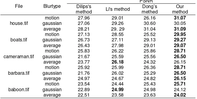
Table 1. quantitative comparative evaluation. PSNR is chosen as performance measure
File Blurtype
gaussian 22.89 24.99 24.98 24.12 average 22.51 23.58 23.63 24.02
*Best results are noted in bold.
The experimental results of deblurred image in terms ofPSNR and SSIM are presented in Table 1 and Table 2 respectively. From the two tables, we can conclude that our algorithm shows superior performance than Dilips’s onboth PSNR and SSIM. From the deblurred image in Figure 1 and Figure 2,there exists noise amplification in smooth regions in Dilips’s method, such as face region in Barbara, background region inHouse and Cameraman. In contrast, our algorithm is able toget more acceptable results on the deblurred images in thesesmooth and
textured regions with fewer ringing effects. Onepossible explanation is that the assumed prior distribution ofedges used in [12],[15],[23] does not hold well whereas our methodexploits the information from the blurred image.
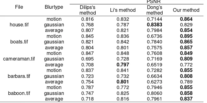
Table 2.quantitative comparative evaluation. SSIM is chosen as performance measure
File Blurtype
PSNR Dilips's
method Li's method
Dong’s
methed Our method
house.tif
motion 0.816 0.832 0.7144 0.864
gaussian 0.768 0.787 0.8383 0.829 average 0.807 0.821 0.7984 0.854
boats.tif
motion 0.845 0.836 0.6736 0.895
gaussian 0.821 0.842 0.7840 0.865
average 0.804 0.801 0.7575 0.857
cameraman.tif
motion 0.847 0.848 0.7608 0.849
gaussian 0.695 0.728 0.7169 0.809
average 0.708 0.797 0.6519 0.772
barbara.tif
motion 0.837 0.841 0.7282 0.855
gaussian 0.723 0.732 0.6634 0.808
average 0.754 0.801 0.6273 0.789
baboon.tif
motion 0.787 0.772 0.7946 0.855
gaussian 0.747 0.825 0.8060 0.858
average 0.718 0.816 0.7961 0.837
*Best results are noted in bold.
(a) (b) (c) (d) (e)
(f) (g) (h) (i) (j)
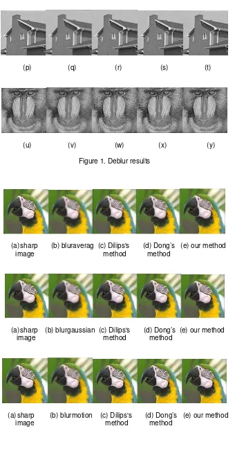
(p) (q) (r) (s) (t)
(u) (v) (w) (x) (y)
Figure 1. Deblur results
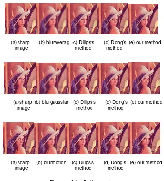
(a) sharp (b) bluraverag (c) Dilips's (d) Dong’s (e) our method image method method
(a) sharp (b) blurgaussian (c) Dilips's (d) Dong’s (e) our method image method method
(a) sharp (b) bluraverag (c) Dilips's (d) Dong’s (e) our method image method method
(a) sharp (b) blurgaussian (c) Dilips's (d) Dong’s (e) our method image method method
(a) sharp (b) blurmotion (c) Dilips's (d) Dong’s (e) our method image method method
Figure 2. Color Deblur results
From Figure 2 and Table 3, we can see that our methodis amuch more effectivedeblurring method. The deblurring results with competing methods are compared in Figure 2. Wecan see that there are many noise residuals and artifacts around edges in the deblurred images in Dilips's method [15].Our method leads to the best visual quality. It not only can remove the blurring effects and noise, but also can reconstruct more and sharper image edges than Dilips's methods.
Table 3. PSNR and SSIM results of deblurring images.
File Blurtype
PSNR SSIM Dilips's
method
Our method
Dilips's method
Our method
Parrot.jpg
motion 22.56 25.76 0.738 0.835
gaussian 23.76 25.89 0.771 0.834
average 22.44 25.34 0.705 0.809
Lena.jpg
motion 25.98 28.61 0.782 0.851
gaussian 25.23 26.93 0.722 0.783
average 24.41 26.74 0.651 0.757
*Best results are noted in bold.
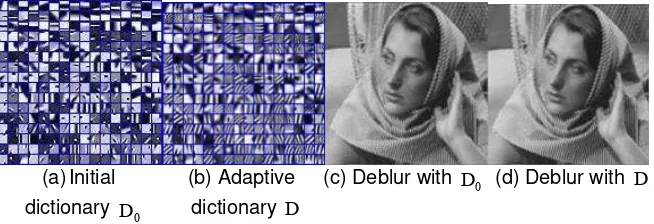
Deblurring withadaptive dictionary is showed the superior performance becauseit exploited the specific information in the image.
(a) Initial (b) Adaptive (c) Deblur with (d) Deblur with dictionary dictionary
Figure 3. Comparison of deblurring results on Barbara with the global learned dictionary and the adaptive dictionary. The PNSR are 25.76dB and 26.50dBrespectively and the SSI are 0.7884
and 0.808
4. Conclusion
In this paper, we proposed an online adaptive dictionarystrategy for image deblurring algorithm based on the sparserepresentation. Our strategy transfers a global learned dictionary to a specific image to make the trade-off between computational cost and accuracy. The new learned dictionary exploited the specific information such as the texture and edge information in the blurred image.Therefore, it can represent patches better than the prespecified dictionary and the global learned dictionary.The approach taken is based onsparse and redundant representations in overcomplete dictionaries learned. With only a few training samples, our methodcan speed up the learning process via domain adaptation. Furthermore, the domain adaptation allows us to circumvent theoverfitting problem effectively. Also, the adaptive dictionaryexploited the specific information in the image, which makes our deblurring algorithm more effective. Experiments havedemonstrated that our image deblurring method yields superiorperformances over other methods.
Acknowledgements
This work was supported Beijing Higher Education Young Elite Teacher Project(NO. YETP1949),Fundamental Research Funds for the Central Universities under Grant No. TD2013-4, and National Natural Science Foundation of China under Grant No. 30901164.
References
[1] R. Fergus, B. Singh, A. Hertzmann, ST. Roweis, WT. Freeman. Removing camera shake from a single photograph. ACM Transactions on Graphics. 2006; 25: 787–794.
[2] A. Levin. Blind motion deblurring using image statistics. Advancesin Neural Information Processing Systems (NIPS). 2006; 2: 4.
[3] Q. Shan, J. Jia, A. Agarwala. High-quality motion deblurring froma single image. ACM Transactions on Graphics. 2008; 27(73):10.
[4] A. Levin, R. Fergus, F. Durand, WT. Freeman. Image and depthfrom a conventional camera with a coded aperture. ACM Transactions on Graphics. 2007; 26: 70-71.
[5] J. Jia. Single image motion deblurring using transparency. Proceedings ofIEEE Conference on ComputerVision and Pattern Recognition. 2007: 1–8.
[6] N. Joshi, R. Szeliski, D. Kriegman. PSF estimation using sharp edgeprediction. Proceedings of IEEE Conference on Computer Vision and Pattern Recognition. 2008: 1–8.
[7] J.-F. Cai, H. Ji, C. Liu, Z. Shen. Blind motion deblurring froma single image using sparse approximation. Proceedings of IEEE Conference on Computer Vision andPattern Recognition. 2009: 104–111.
[8] A. Levin, Y. Weiss, F. Durand, WT. Freeman. Understandingand evaluating blind deconvolution algorithms. Proceedings of IEEE Conference on Computer Vision andPattern Recognition. 2009:
0
D D
0
1964–1971.
[9] N. Joshi, C. Zitnick, R. Szeliski, D. Kriegman. Image deblurringand denoising using color priors. Proceedings of IEEE Conference on Computer Vision and Pattern Recognition. 2009: 1550–1557.
[10] D. Krishnan, R. Fergus. Fast image deconvolution using hyperlaplacian priors. Advances in Neural Information Processing Systems (NIPS). 2009; 22: 1–9.
[11] C. Jia, B. Evans. Patch-based image deconvolution via joint modeling of sparse priors. Proceedings of the 18th IEEE International Conference on image Processing (ICIP). 2011: 681–684.
[12] H. Li, Y. Zhang, H. Zhang, Y. Zhu, J. Sun. Blind image deblurring based on sparse prior of dictionary pair. Proceedings of the 21th International Conference on Pattern Recognition (ICPR). 2012: 3054– 3057.
[13] M. Aharon, M. Elad, A. Bruckstein. K-SVD: An algorithm for designing over complete dictionaries for sparse representation. IEEE Transactions on Signal Processing. 2006; 54: 4311–4322.
[14] Z. Hu, J.B. Huang, M.H. Yang. Single image deblurring with adaptive dictionary learning. Proceedings of the 17th IEEE International Conference on Image Processing (ICIP). 2010: 1169–1172.
[15] K. Dilip, F. Tay, T.and Rob. Blind deconvolution using a normalized sparsity measure. Proceedings of IEEE Conference on Computer Vision and Pattern Recognition(CVPR). 2011: 233–240.
[16] JL. Starck, MK. Nguyen, F. Murtagh. Wavelets and curvelets forimage deconvolution: a combined approach. Signal Processing. 2003; 83: 2279 – 2283.
[17] SS. Chen, DL. Donoho, MA. Saunders. Atomic decompositionby basis pursuit. SIAM journal on scientific computing. 1998; 20: 33–61.
[18] P. Tseng. On accelerated proximal gradient methods for convex-concave optimization. SIAM Journal on Optimization. 2008.
[19] S. Ji, J. Ye. An accelerated gradient method for trace norm minimization. Proceedings of International Conference on Machine Learning. 2009: 457-464.
[20] Y. Lou, A. L. Bertozzi, S. Soatto. Direct sparse deblurring. Journal of Mathematical Imaging and Vision. 2011; 39: 1–12.
[21] J. Mairal, F. Bach, J. Ponce, G. Sapiro. Online dictionary learning for sparse coding. Proceedings of the 26th Annual InternationalConference on Machine Learning. 2009: 689–696.
[22] Z. Wang, AC. Bovik, HR. Sheikh, EP. Simoncelli. Imagequality assessment: from error visibility to structural similarity. IEEE Transactions on Image Processing. 2004; 14: 600–612.