Corresponding Author: S.H. Yahaya, Faculty of Manufacturing Engineering, Universiti Teknikal Malaysia Melaka, 76100 Hang Tuah Jaya, Melaka, Malaysia
G
2Bézier-Like Cubic as the S-Transition and C-Spiral Curves and Its Application in
Designing a Spur Gear Tooth
1
S.H. Yahaya, 2J.M. Ali, 2M.Y. Yazariah, 1Haeryip Sihombing and 1M.Y. Yuhazri
1
Faculty of Manufacturing Engineering, Universiti Teknikal Malaysia Melaka, 76100 Hang Tuah Jaya, Melaka, Malaysia
2
School of Mathematical Sciences, Universiti Sains Malaysia, 11800 Minden, Pulau Pinang, Malaysia
Abstract: Many of the researchers or designers are mostly used the involute curves (known as one of the approximation curves) to design the profile of gears. This study intends to develop the transition (S transition and C spiral) curves using Bézier–like cubic curve function with G2 (curvature) continuity as the degree of smoothness. Method of designing the transition curves is adapted by using circle to circle templates. While the transition curves are completely finished, it will be applied in redesigning the profile of spur gear. The mathematical proofs and simple models are also shown.
Key words: Spur gear profile; Transition curve; Spiral curve; G2 continuity
INTRODUCTION
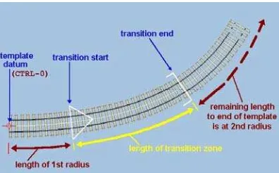
Fig. 1: Railways Route Design Modeling Using Transition Curves (Yellow Color) Application (Martin, 2013)
Fig. 2: Third (Left) and Fifth (Right) Cases of Circle to Circle Templates (Baass, 1984; Walton and Meek, 1996; Meek and Walton, 1989)
Notations and Convections:
Consider the Euclidean system such as vectors, A(Ax,Ay)and B
(Bx,
By). The norm of the vector is defined as A Ax2Ay2.
The derivative of a function, f is represented as f.
Let the dot product of two vectors, A and B is expressed as AB while the cross product of vectors is expressed as A^B.A planar of parametric curve is defined by a set of points, z(t)(x(t),y(t)) where t in the real interval. In this paper, the interval of t applied is t[0,1]. Following the approaches of Juhász (1998) and Artin (1957), we can simplify the dot and cross product to
x y y x
y y x x
B A B A
B A B A
) sin( ^
) cos(
B A B A
B A B A
(1) where, is an anti-clockwise angle. The tangent vector of a plane parametric curve is denoted as z(t).If
, 0 ) ( t
z the expression of curvature, (t)can be expressed as (Hoschek and Lasser, 1993; Faux and Pratt, 1988)
3 ) (
) ( )^ ( ) (
t z
t z t z t
(2)
and its derivative expanded as 5
) (
) ( ) (
t z
t t
(3)
)}
Next, we will discuss the applications of parametric function, namely a Bézier-like cubic curve which will be used in this study.
Bézier-Like Cubic Curve:
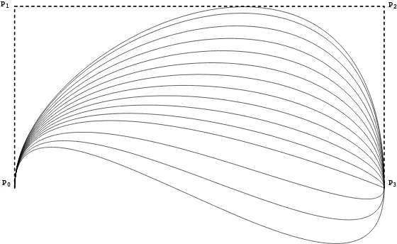
Bézier-like cubic curve (also known as cubic Alternative curve) is a new basis function in the field of Computer Aided Geometric Design (CAGD). Bézier-like basis function simplifies the process of controlling the curve since it has only two shape parameters, λ0 and λ1 to control or change the shape of the curve such in Figures 3 and 4, compared to cubic Bézier curve for which the control points needs to be adjusted (Farin, 1997). Bézier-like cubic curve is formulated by applying the form of Hermite interpolation given by (Ali, 1994; Ali et al., 1996; Ahmad, 2009)
are Bézier-like cubic basis
functions. Hence, Bézier-like cubic curve can be written as
3 whereas when λ0 = λ1= 3, they will become a cubic Bernstein Bézier basis functions and cubic Trimmer basis functions if the shape values equal to 4.
P3
P2
P1
P0
In the next section, we will explore the control points identification in Bézier-like cubic curve based on circle to circle template (Figure 2).
Circle to Circle Templates:
a. Third Case of Circle Template as an S-Shaped Transition Curve:
Cubic Bézier curve had been predominantly used in curve design, as shown in studies by Habib and Sakai (2003) and Walton and Meek (1999). The similarity between this function and Bézier-like cubic curve is that both functions have four control points. In circle to circle problems, polar coordinate system is usually selected because of its direct relation to the polar angle and thus is easier to implement. This coordinate system is shown in Figure 5.
Fig. 5: Polar Coordinate in Cartesian Vector System (Anwane, 2007) By referring to Habib and Sakai (2003), the control points are stated as
} control points are unique only in the case of S-shaped transition curve. The improvements are made in (7) to increase the degree of freedom and its applicability such
} parameters remain the same as in (7). The value of h and k will be calculated by using the curvature continuous (G2 continuity) shown as
This continuity measures position, direction, and radius of curvature at the ends such as the following curve illustrated in Figure 6. The details of obtaining the value of h and k will be discussed in Section 5. By applying these theories, an S-shaped curve is demonstrated in Figure 7.
c0
r0
P0
P1
P3
P2
c1 r1
k
h
P2, P1 0
1
Fig. 7: An S-Shaped Transition Curve Produced by Using G2 Bézier-Like Cubic Curve
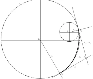
b. Fifth Case of Circle Template as a Spiral C-Transition Curve:
The fifth case will produce a type of C-shaped transition curve as a single spiral (Baass, 1984; Walton and Meek, 1996; Habib and Sakai, 2005). Generally, transition curve is a special curve where the degree of curvature is varied to give a gradual transition between a tangent and a simple curve or between two simple curves at the point of connection. Single spiral is defined as a plane curve with monotone curvature function or the term “spiral” in the sense of monotonicity of curvature (Kurnosenko, 2009). In addition, the curvature is continuous and has a constant sign which lead to either the curvature is strictly increasing or decreasing (Kurnosenko, 2009; Ghomi, 2007)
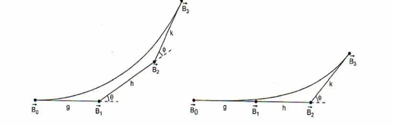
Fig. 8: Transition (Left) and Spiral (Right) Curves Architecture Applied in Cubic Bézier Curve (Walton et al., 2003)
The curve architecture in transition and spiral curves is totally different from the segmentations used. As shown in Figure 8, three segments are needed to design C-shaped transition curve whereas only two segments are used in C spiral curve. We now identify the control points as in (Habib and Sakai, 2003)
} cos , {sin *
}, sin , {cos *
} cos , sin { *
}, sin , {cos *
3 2 1
1 3
0 1 0
0 0
k P P r
c P
h P P r
c P
} to design C spiral curve, the segments used in (11) should be reduced (Walton et al., 2003) by assuming that
2
1 P
P (12) Then, in (12) either h or k can be eliminated by using a dot product. If the parameter chosen is k, the expression will be dotted with a vector, {cos,sin} where
The modified control points that satisfy the fifth case template (C spiral curve) are given by
}
In order to join C spiral curve with the circles, we will need to apply the curvature continuity such
1
This continuity is also used to determine the shape parameters, λ0 and λ1 in (6). The determination of both parameters will be considered in the next section. A generated C-shaped curve is visualized in Figure 9.
P0
Fig. 9: C-Shaped Curve in Fifth Case of Circle Templates Using G2 Bézier-Like Cubic Curve
Curvature Analysis:
a. The Analyzing of Curvature in Third Case of Circle Template:
chosen to be {2.5, 1.8} (0, 3) as the stability and positive conditions is obtained in this range (Figure 4). The radii are found to be r0 = r1 = 0.206 and as a result, h and k are equivalent to 0.2779 and 0.3780 using (6), (8) and (9). The extension is needed to identify the curvature extreme that may exist in this S curve design. We write (3) in the form of where (t) and (t) are both functions that have t as independent variables. The function, (t) has a complex form and difficult to find out the curvature extreme. For the existence in (16), the condition should be
0 ) (t
(17) Mathematically, (t) is a function that totally dominates the whole functions in (16). By considering this reason, the curvature extreme will be determined by applying the profile of function, (t) such
F arc length of this case (Walton and Meek, 1996; Rashid and Habib, 2010). The formulation of arc length, S is demonstrated as By applying (20) and curvature profile in (2) according to the inputs above, then S = 0.61507. Therefore, an interval of t used for analysis purposes is [0, 0.61507]. Equation (19) is set to zero to obtain the critical numbers where
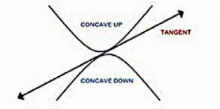
In the list of critical numbers in (21), the first two terms are selected to satisfy the new region of t. The critical numbers of t are 0.2250 and 0.4706. We will extend this study to find whether these two critical numbers have either minimum curvature extreme or maximum curvature extreme. The methods that can be employed are Second Derivative and Concavity Tests (Stewart, 2003) (Figure 10).
Definition 1:
The second derivative test is said to have a relative minimum at point, x0 if f(x0)0 while a relative maximum iff(x0)0. In the case off(x0)0, the graph is increasing (concave upward) or in concave downward (decreasing) if f(x0)0 as explained in concavity test (Stewart, 2003).
Fig. 10: A Set of Graphs Clustered in Concavity Test (Stewart, 2003) Hence, the derivative of (19) gives an expansion of
Q
0.1 0.2 0.3 0.4 0.5 0.6 ArcLength
5 4 3 2 1 1 2 t
0.1 0.2 0.3 0.4 0.5 0.6 ArcLength
5 5 10 15 20
1 t
Fig. 11: Curvature Profile, (t) (Left) and Its Derivative, (1) (t) (Right) along Interval 0 t S in Third Case of
Circle Template, S-Shaped Transition Curve
Theorem 1:
An S-shaped transition curve generated by using G2 Bézier-like cubic curve as a function is guaranteed to have two curvature extrema with one curvature inflection point as λ0 and λ1 are in (0, 3) and where h and k are calculated by using G2 continuity on the interval, t [0, S].
b. The Analyzing of Curvature in Fifth Case of Circle Template:
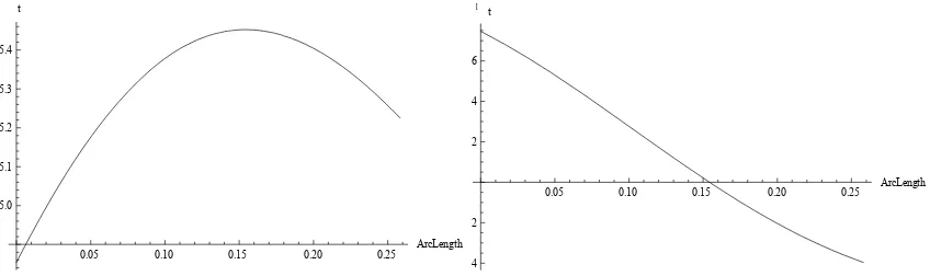
Based on Kneser’s theorem (Guggenheimer, 1963), a transition curve cannot be a type of spiral arc. However, it may have at least one interior curvature extreme. Therefore, the analysis is focused on the transition curve that has exactly one interior curvature extreme and is free of inflection points, loops and cusps (Habib and Sakai, 2008; Habib and Sakai, 2003). These will show that (3) only has one zero on 0 t S (Habib and Sakai, 2008). We can proceed by choosing c0 = {-0.398, 0.689} and c1 = {-0.247, 0.725} with the angles, β [0.5π, π) = 0.6667π radian and α (0, 0.5π) = 0.05556π radian. The radii are chosen to be r0 = 0.206 and r1 = 0.05. Hence, k is calculated by using (13) and its value is 0.1431 with shape parameters, {λ0, λ1} are estimated by employing (2), (6), (12), (14) and (15). As a result, we found that λ0 = 2.7695 and λ1 = 0.3619 approximately. By applying (3) with all the inputs, it will be simplified similar to (16) and (17) as the existence condition. The equation of (t) is given by
F t E t D t C t B t A
t) * * * * *
( 5 4 3 2
(24)
where A = -2.9037, B = 11.8210, C = -18.3709, D = 13.2609, E = -4.1989 and F = 0.3932. Then, we would like to find out the zeros by setting
0 ) (t
(25) Therefore, the result is shown in the list such
,...} 0723 . 1 , 6918 . 0 , 1543 . 0 , 15 0583 . 1
{ E
t (26)
As explained above, the range of t is between zero to arc length, S. In this C-shaped case, S is calculated as 0.2583 by applying (2) and (20). In (26), only second value satisfies the interval of t [0, 0.2583]. Thus, we can say that only one zero exists definitely on the interval, t [0, S]. By this proofing, a C shaped curve has shown that only one interior curvature extreme exists on 0 t S. This proof can be seen clearly in Figure 12. Both of these curve theories will be applied to redesign a profile (tooth) of spur gear. Currently, an involute or evolute curve is always used in designing this spur tooth profile.
0.05 0.10 0.15 0.20 0.25 ArcLength
5.0 5.1 5.2 5.3 5.4 t
0.05 0.10 0.15 0.20 0.25 ArcLength
4 2 2 4 6 1t
Fig. 12: Curvature profile, (t) (Left) and Its Derivative, (1) (t) (Right) along Interval 0 t S in Fifth Case of
Theorem 2:
A C-shaped transition curve generated by using G2 Bézier-like cubic curve as a spiral curve if and only if the fifth case of circle template is applied where k and shape parameters, λ0, λ1 are determined by using P1 = P2 and G2 continuity on the interval, t [0, S].
Spur Gear Tooth Design: a. Definition of spur gear:
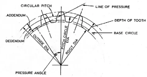
Traditional spur gears have the teeth which are straight and parallel to the axis of shaft that conveys the gear (Mott, 2003). Normally, the teeth have an involute form where this form can be acted as in contacting the teeth (Mott, 2003). Figure 13 shows a schematic and related terminology for spur gear.
Fig. 13: Some of the Terms in Spur Gear (Price, 1995)
Based on Figure 13, an inner circle and an outer circle can be drawn and smaller circles can be fitted within their boundaries, as shown in Figure 14. This resulting structure will be used to design a profile (tooth) of spur gear.
Fig. 14: A New Basis Model of Designing a Spur Gear Tooth
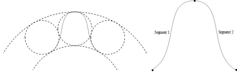
b. Single Tooth Design Using Third Case of Circle Template:
Segment 1 Segment 2
.
.
.
Fig. 15: Single Tooth of Spur Gear Using Third Case of Circle Templates (Left) and Its Segmentation (Right)
c. Single Tooth Design Using Fifth Case of Circle Templates:
In this case, Figure 14 is modified to suit the elements in fifth case of circle templates. The small circles are drawn at the intersection of two circles. For this template, it needs four segments to design a single tooth of spur gear. Segment one consists of c0 = {-0.398, 0.689}, c1 = {-0.247, 0.725}, α = 0.05556π radian, β = 0.6667π radian, r0 = 0.206 and r1 = 0.05. The values of k and shape parameters, λ0, λ1 are computed by using (2), (6), (11), (13) and (15). We found that k = 0.1431 whereas λ0 and λ1 are equal to 2.7695 and 0.3619, respectively. For segment two, the inputs are c0 = {0, 0.795}, c1 = {-0.247, 0.725}, β = 1.5π radian while the rest are exactly the same as in segment one. This time, k and shape parameters, λ0, λ1 are found to be 0.2449, 2.1279 and 0.5343, respectively.
These two segments have a symmetrical curve which can be defined as mirroring or balancing to segment three and four. Thus, segment three and four have similar shape to segment one and two, respectively (Du Sautoy, 2009). Figure 16 shows the design of the tooth and its segmentation using fifth case of circle templates. The comparison of the curve segmentation produced from these two different cases (third and fifth) is shown in Figure 17.
.
.
.
.
.
Segment 1 Segment 2
Segment 4
Segment 3
Fig. 16: Single Tooth of Spur Gear Using Fifth Case of Circle Templates (Left) and Its Segmentation (Right)
.
.
.
.
.
Next, we will apply the single tooth designs using third and fifth cases of circle templates in order to develop a solid model of spur gear.
Solid of Spur Gear:
In Computer Aided Geometric Design (CAGD), the technique commonly used such surface design where in this design technique, several properties need to be considered (Bloor et al., 1995), difficult to extrude as a solid model and not suitable in Computer Aided Analysis (CAE) purposes. To solve these problems, the application of approximation theory is used by employing the method of selection points (coordinates) to redesign and remain the same profiles shown in Figures 15 and 16. The points will be selected along the curve in both figures. Notice that, the more points that are selected, the generated curve or model will have better accuracy (less error) (Mathews and Fink, 2004). For this purpose, we will use Wolfram Mathematica 7.0. The detailed explanation about these procedures will be discussed in the next subsection.
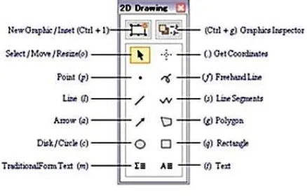
a. Coordinate Selection Using Wolfram Mathematica 7.0:
Wolfram Mathematica 7.0 has many accessibility features such drawing tools in taskbar of graphics. One of these tools is “get coordinates” which is used to mark the coordinates in 2D graphics or 2D plots. By applying this tool together with the mouse pointer moves over the plots, the approximate coordinate value is then displayed. Then, click to mark the coordinate. In order to have more markers (coordinates), click to other position in the plots. Explanation for these procedures is visualized in Figures 18 and 19.
Fig. 18: Drawing Tools in Wolfram Mathematica 7.0 (Wagon, 2010)
Fig. 19: “Get Coordinates” Tool and Its Related Example
Finally, copy the marked coordinates (Figure 19) and paste these coordinates into an input cell in Mathematica. The list of coordinates extracted from the plot is shown in Figure 20.
0.2516, 0.8679 , 0.3606, 1.052 , 0.4864, 1.229 , 0.6205, 1.388 , ...
Figure 20: An Example of Coordinates Extracted from 2D Plot or Curve
b. S and C Shaped as the Curves in Solid of Spur Gear:
problems above are then discovered. There are 34 coordinates have been chosen for both curves. The following process flow diagram is used to redesign the profile of spur gear in accordance to these coordinates (Figure 21). Two models of six gear teeth are developed with the outside and shaft diameters are 70 mm and 19 mm. Figure 22 shows spur gear models using both curves following the diagram in Figure 21. In addition, the developed models are suitable for enhancement in oil pump application compared to the existing profiles (Figure 23). However, future analysis must be done to investigate and fully understand this applicability.
Fig. 21: Process Flow Diagram Applied in Developing a Solid of Spur Gear
Fig. 22: Solid of Spur Gear Using S (Left) and C (Right) Shaped Curves
Fig. 23: One of the Existing Models in Oil Pumps (Sasaki et al., 2008)
Conclusion:
This paper proposes the designing of S (third case) and C (fifth case) templates or known as the parameterized (transition and spiral) curves using a function of Bézier-like cubic curve with curvature continuity smoothness. The proofing of these two curves in accordance to concavity and second derivative tests was also shown. By the integrated use of Wolfram Mathematica 7.0 and CATIA V5, highly accurate profiles of spur gear teeth with S and C-shaped curves were obtainable as Computer Aided Design (CAD) model, with smoother profile as compared to existing gear teeth (Figure 23). The resulting solid CAD model of the gear can be analyzed using finite element and acoustic methods for performance evaluation.
Coordinates definition
Joint the coordinates
Extrude Process 2D model Spline
package
ACKNOWLEDGEMENT
This research was supported by Universiti Teknikal Malaysia Melaka under the Fundamental Research Grant Scheme (FRGS). The authors gratefully acknowledge everyone who contributed helpful suggestions comments.
REFERENCES
Ahmad, A., 2009. Parametric spiral and its application as transition curve, Ph.D. thesis, Universiti Sains Malaysia, PG.
Ali, J.M., 1994. An Alternative Derivation of Said Basic Function. Sains Malaysiana, 23: 42-56.
Ali, J.M., H.B. Said, and A.A. Majid, 1996. Shape Control of Parametric Cubic Curves. In the Proceedings of the Fourth International Conference on Computer-Aided Design and Computer Graphics, China, pp: 128-133. Anwane, S.W., 2007. Chapter I: Vector analysis, Polar coordinate system. In: Fundamentals of electromagnetic fields, USA: Infinity Science Press.
Artin, E., 1957. Geometric Algebra. New York: Interscience.
Baass, K.G., 1984. The Use of Clothoid Templates in Highway Design. Transportation Forum, 1: 47-52. Babu, V.S., and A.A. Tsegaw, 2009. Involute Spur Gear Template Development by Parametric Technique Using Computer Aided Design. African Research Review, 3(2): 415-429.
Bloor, M.I.G., M.J. Wilson, and H. Hagen, 1995. The Smoothing Properties of Variational Schemes for Surface Design. Computer Aided Geometric Design, 12(4): 381-394.
Bradford, L.J. and G.L. Guillet, 1943. Kinematics and Machine Design. New York: John Wiley & Sons. Du Sautoy, M., 2009. Symmetry: A Journey into the Patterns of Nature. UK: HarperCollins.
Farin, G., 1997. Curves and Surfaces for Computer Aided Geometric Design, a Practical Guide, Fourth Ed. New York: Academic Press.
Faux, I.D. and M.J. Pratt, 1988. Computational Geometry for Design and Manufacture. Chichester: Ellis Horwood Ltd.
Ghomi, M., 2007. Volume I: Curves and surfaces, Math 4441. In: Differential geometry module, Georgia Tech.
Guggenheimer, H., 1963. Differential Geometry. New York: McGraw-Hill.
Habib, Z., and M. Sakai, 2008. G2 Cubic Transition between Two Circles with Shape Control. Journal of Computational and Applied Mathematics, 223: 133-144.
Habib, Z., and M. Sakai, 2003. G2 Planar Cubic Transition between Two Circles. International Journal of Computer Mathematics, 8: 959-967.
Habib, Z., and M. Sakai, 2005. Circle to Circle Transition with a Single Cubic Spiral. In the Proceedings of the Fifth IASTED International Conference Visualization, Imaging and Image Processing, Spain, pp: 691-696.
Habib, Z., and M. Sakai, 2003. Family of G2 Spiral Transition between Two Circles. In the Proceedings of the Advances in Geometric Modeling, M. Sarfraz (Eds.). New York: John Wiley & Sons, pp: 133-150.
Hoschek, J., and D. Lasser, 1993. Fundamentals of Computer Aided Geometric Design (Translation by L. L. Schumaker). Massachusetts: A.K. Peters Wellesley.
Juhász, I., 1998. Cubic Parametric Curves of Given Tangent and Curvature. Journal of Computer Aided Design, 25: 1-9.
Kurnosenko, A.I., 2009. General Properties of Spiral Plane Curves. Journal of Mathematical Sciences, 161: 405-418.
Martin, W., 2013. A Little Gentle Geometry. UK: Templot.
Mathews, J.H. and K.D. Fink, 2004. Numerical Methods Using MATLAB, Fourth Ed. USA: Pearson Prentice Hall.
Meek, D.S., and D.J. Walton, 1989. The Use of Cornu Spirals in Drawing Planar Curves of Controlled Curvature. Journal of Computational and Applied Mathematics, 25: 69-78.
Mott, R.L., 2003. Machine Elements in Mechanical Design Fourth Edition. New Jersey: Prentice Hall. Price, D., 1995. Spur gears. In: Mechanical engineering design topics, GlobalSpec.
Rashid, A., and Z. Habib, 2010. Gear Tooth Designing with Cubic Bézier Transition Curve. In the Proceedings of the Graduate Colloquium on Computer Sciences (GCCS), Lahore, pp: 1-5.
Rashid, A., and Z. Habib, 2010. Smoothing Arc Splines Using Cubic Bézier Spiral. In the Proceedings of the Graduate Colloquium on Computer Sciences (GCCS), Lahore, pp: 6-15.
Sasaki, H., N. Inui, Y. Shimada and D. Ogata, 2008. Development of High Efficiency P/M Internal Gear Pump Rotor (Megafloid Rotor). Sei Technical Review, 66: 124-128.
Stewart, J., 2003. Calculus, Fifth Ed. Belmont CA: Thomson Brooks/Cole.
Walton, D.J., and D.S. Meek, 1999. Planar G2 Transition between Two Circles with Fair Cubic Bézier Curve. Computer Aided Design, 31: 857-866.
Walton, D.J., and D. S. Meek, 1996. A Planar Cubic Bézier Spiral. Journal of Computational and Applied Mathematics, 72: 85-100
Walton, D.J., D.S. Meek and J.M. Ali, 2003. Planar G2 Transition Curves Composed of Cubic Bézier Spiral Segments. Journal of Computational and Applied Mathematics, 157: 453-476.