QUANTITATIVE TRAIT LOCI MAPPING FOR TRAIT
IN BINARY AND ORDINAL SCALE
FARIT MOCHAMAD AFENDI
GRADUATE SCHOOL
BOGOR AGRICULTURAL UNIVERSITY
BOGOR
ABSTRACT
FARIT MOCHAMAD AFENDI. Quantitative Trait Loci Mapping for Trait in Categorical Scale. Under the direction of Asep Saefuddin, Muhammad Jusuf, and Totong Martono.
Genes or regions on chromosome underlying a quantitative trait are called Quantitative Trait Loci (QTL). Characterizing genes controlling quantitative trait on their position in chromosome and their effect on trait is through a process called QTL mapping. In estimating the QTL position and its effect, QTL mapping basically utilize the association between QTL and DNA markers. However, many important traits are obtained in categorical scale, such as resistance from certain disease. From a theoretical point of view, QTL mapping method assuming continuous trait could not be applied to categorical trait.
This research was focusing on the assessment of the performance of Maximum Likelihood (ML) and Regression (REG) approach employed in QTL mapping as well as the performance of Lander and Botstein (LB) and Piepho method in determining critical value in testing the existence of QTL for binary and ordinal trait by means of simulation study. The simulation study to evaluate the performance of ML and REG approach was conducted by taking into account several factors that may affecting the performance of both approaches. The factors are: (1) marker density; (2) QTL effect; (3) sample size; (4) shape of phenotypic distribution; (5) number of categories; and (6) number of QTL. Moreover, the simulation study for evaluating LB and Piepho method in determining critical value was conducted by generating distribution of the test statistic under null hypothesis.
approach in QTL mapping analysis for binary trait, the two approaches showing comparable performance; whereas for ordinal trait REG approach showing poor performance compared with ML approach in estimating thresholds. As a result, in QTL mapping analysis, ML and REG approach could be used when dealing with binary trait, whereas ML approach is suggested when dealing with ordinal trait.
ABSTRAK
FARIT MOCHAMAD AFENDI. Quantitative Trait Loci Mapping for Trait in Categorical Scale. Dibimbing oleh Asep Saefuddin, Muhammad Jusuf, dan Totong Martono.
Gen atau suatu segmen di kromosom yang mendasari sifat kuantitatif dinamakan dengan Lokus Sifat Kuantitatif (Quantitative Trait Loci/QTL). Penelusuran gen yang mengatur sifat kuantitatif dalam hal posisinya di kromosom serta besar pengaruhnya dilakukan melalui proses yang dinamakan pemetaan QTL. Di dalam menduga posisi QTL dan besar pengaruhnya, pemetaan QTL pada dasarnya memanfaatkan hubungan antara QTL dengan penanda DNA. Di sisi lain, banyak sifat penting lain yang diamati dengan skala kategorik seperti ketahanan terhadap suatu penyakit. Secara teori, metode pemetaan QTL dengan anggapan sifat kontinu tidak dapat diterapkan pada sifat kategorik.
Penelitian ini bertujuan untuk menilai performa metode kemungkinan maksimum (ML) dan regresi (REG) yang diterapkan pada pemetaan QTL dan performa metode Lander dan Botstein (LB) dan Piepho di dalam penentuan titik kritis untuk pengujian keberadaan QTL untuk sifat dengan skala biner dan ordinal dengan menggunakan simulasi. Kajian simulasi untuk mengevaluasi performa metode ML dan REG dilakukan dengan memperhatikan beberapa faktor yang mungkin mempengaruhi performa kedua sifat ini. Faktor-faktor tersebut adalah: (1) kepadatan penanda; (2) besar pengaruh QTL; (3) ukuran contoh; (4) bentuk sebaran fenotipe; (5) banyaknya kategori; dan (6) banyaknya QTL. Selanjutnya, kajian simulasi untuk menilai performa metode LB dan Piepho di dalam penentuan titik kritis dilakukan dengan membangkitkan sebaran statistik uji di bawah hipotesis nol.
kedua metode menunjukkan performa yang serupa; sedangkan untuk sifat ordinal metode REG menunjukkan performa yang kurang dibandingkan metode ML terutama di dalam menduga titik ambang (threshold). Dengan demikian, metode ML dan REG dapat digunakan untuk sifat biner, sedangkan untuk sifat ordinal metode ML yang disarankan.
LETTER OF PRONOUNCEMENT
With this I stated that my thesis which is entitled:
Quantitative Trait Loci Mapping for Trait in Binary and Ordinal Scale is based on my own research and never published before. All of the data source and information has been stated clearly and could be reviewed.
Bogor, August 2006
QUANTITATIVE TRAIT LOCI MAPPING FOR TRAIT
IN BINARY AND ORDINAL SCALE
FARIT MOCHAMAD AFENDI
A Thesis submitted to the Graduate School of Bogor Agricultural University
in partial fulfillment of the requirements for the degree of
Master of Science
GRADUATE SCHOOL
BOGOR AGRICULTURAL UNIVERSITY
BOGOR
Copyright © 2006 by Bogor Agricultural University All rights reserved
No part of this thesis may be reproduced, stored in a retrieval system, or transcribed, in any form or by any means – electronic, mechanical, photocopying, recording, or
Title : Quantitative Trait Loci Mapping for Trait in Binary and Ordinal Scale
Name : Farit Mochamad Afendi
NRP : G151030091
Study Program : Statistics
Approved by, 1. Advisory Committee
Dr. Ir. Asep Saefuddin Chair
Dr. Ir. Muhammad Jusuf Dr. Ir. Totong Martono
Co-chair Co-chair
Acknowledged by,
2. Chair of Study Program of Statistics 3. Dean of Graduate School
Dr. Ir. Aji Hamim Wigena Dr. Ir. Khairil Anwar Notodiputro, M.S.
QUANTITATIVE TRAIT LOCI MAPPING FOR TRAIT
IN BINARY AND ORDINAL SCALE
FARIT MOCHAMAD AFENDI
GRADUATE SCHOOL
BOGOR AGRICULTURAL UNIVERSITY
BOGOR
ABSTRACT
FARIT MOCHAMAD AFENDI. Quantitative Trait Loci Mapping for Trait in Categorical Scale. Under the direction of Asep Saefuddin, Muhammad Jusuf, and Totong Martono.
Genes or regions on chromosome underlying a quantitative trait are called Quantitative Trait Loci (QTL). Characterizing genes controlling quantitative trait on their position in chromosome and their effect on trait is through a process called QTL mapping. In estimating the QTL position and its effect, QTL mapping basically utilize the association between QTL and DNA markers. However, many important traits are obtained in categorical scale, such as resistance from certain disease. From a theoretical point of view, QTL mapping method assuming continuous trait could not be applied to categorical trait.
This research was focusing on the assessment of the performance of Maximum Likelihood (ML) and Regression (REG) approach employed in QTL mapping as well as the performance of Lander and Botstein (LB) and Piepho method in determining critical value in testing the existence of QTL for binary and ordinal trait by means of simulation study. The simulation study to evaluate the performance of ML and REG approach was conducted by taking into account several factors that may affecting the performance of both approaches. The factors are: (1) marker density; (2) QTL effect; (3) sample size; (4) shape of phenotypic distribution; (5) number of categories; and (6) number of QTL. Moreover, the simulation study for evaluating LB and Piepho method in determining critical value was conducted by generating distribution of the test statistic under null hypothesis.
approach in QTL mapping analysis for binary trait, the two approaches showing comparable performance; whereas for ordinal trait REG approach showing poor performance compared with ML approach in estimating thresholds. As a result, in QTL mapping analysis, ML and REG approach could be used when dealing with binary trait, whereas ML approach is suggested when dealing with ordinal trait.
ABSTRAK
FARIT MOCHAMAD AFENDI. Quantitative Trait Loci Mapping for Trait in Categorical Scale. Dibimbing oleh Asep Saefuddin, Muhammad Jusuf, dan Totong Martono.
Gen atau suatu segmen di kromosom yang mendasari sifat kuantitatif dinamakan dengan Lokus Sifat Kuantitatif (Quantitative Trait Loci/QTL). Penelusuran gen yang mengatur sifat kuantitatif dalam hal posisinya di kromosom serta besar pengaruhnya dilakukan melalui proses yang dinamakan pemetaan QTL. Di dalam menduga posisi QTL dan besar pengaruhnya, pemetaan QTL pada dasarnya memanfaatkan hubungan antara QTL dengan penanda DNA. Di sisi lain, banyak sifat penting lain yang diamati dengan skala kategorik seperti ketahanan terhadap suatu penyakit. Secara teori, metode pemetaan QTL dengan anggapan sifat kontinu tidak dapat diterapkan pada sifat kategorik.
Penelitian ini bertujuan untuk menilai performa metode kemungkinan maksimum (ML) dan regresi (REG) yang diterapkan pada pemetaan QTL dan performa metode Lander dan Botstein (LB) dan Piepho di dalam penentuan titik kritis untuk pengujian keberadaan QTL untuk sifat dengan skala biner dan ordinal dengan menggunakan simulasi. Kajian simulasi untuk mengevaluasi performa metode ML dan REG dilakukan dengan memperhatikan beberapa faktor yang mungkin mempengaruhi performa kedua sifat ini. Faktor-faktor tersebut adalah: (1) kepadatan penanda; (2) besar pengaruh QTL; (3) ukuran contoh; (4) bentuk sebaran fenotipe; (5) banyaknya kategori; dan (6) banyaknya QTL. Selanjutnya, kajian simulasi untuk menilai performa metode LB dan Piepho di dalam penentuan titik kritis dilakukan dengan membangkitkan sebaran statistik uji di bawah hipotesis nol.
kedua metode menunjukkan performa yang serupa; sedangkan untuk sifat ordinal metode REG menunjukkan performa yang kurang dibandingkan metode ML terutama di dalam menduga titik ambang (threshold). Dengan demikian, metode ML dan REG dapat digunakan untuk sifat biner, sedangkan untuk sifat ordinal metode ML yang disarankan.
LETTER OF PRONOUNCEMENT
With this I stated that my thesis which is entitled:
Quantitative Trait Loci Mapping for Trait in Binary and Ordinal Scale is based on my own research and never published before. All of the data source and information has been stated clearly and could be reviewed.
Bogor, August 2006
QUANTITATIVE TRAIT LOCI MAPPING FOR TRAIT
IN BINARY AND ORDINAL SCALE
FARIT MOCHAMAD AFENDI
A Thesis submitted to the Graduate School of Bogor Agricultural University
in partial fulfillment of the requirements for the degree of
Master of Science
GRADUATE SCHOOL
BOGOR AGRICULTURAL UNIVERSITY
BOGOR
Copyright © 2006 by Bogor Agricultural University All rights reserved
No part of this thesis may be reproduced, stored in a retrieval system, or transcribed, in any form or by any means – electronic, mechanical, photocopying, recording, or
Title : Quantitative Trait Loci Mapping for Trait in Binary and Ordinal Scale
Name : Farit Mochamad Afendi
NRP : G151030091
Study Program : Statistics
Approved by, 1. Advisory Committee
Dr. Ir. Asep Saefuddin Chair
Dr. Ir. Muhammad Jusuf Dr. Ir. Totong Martono
Co-chair Co-chair
Acknowledged by,
2. Chair of Study Program of Statistics 3. Dean of Graduate School
Dr. Ir. Aji Hamim Wigena Dr. Ir. Khairil Anwar Notodiputro, M.S.
BIOGRAPHY
As the last children from sixth brother of my family, I was born to my father H. Abdus Syakur Suyitno (alm) and my mother Hj. Siti Aisyah in 1979 in Jepara, a city which well known on its wood carving and birthplace of Kartini.
ACKNOWLEDGEMENTS
Alhamdulillah. That is my first word as my thanks to Allah, God The Almighty. Without Him, I will unable to do anything.
I would like to thank my first advisor Dr. Asep Saefuddin who encourages me to brave writing paper in English since my undergraduate. I thank my second advisor Dr. Muhammad Jusuf for give me the first sight in application of statistics in genetics and for keep me enrich the biology concept in my research. I also thank to my third advisor Dr. Totong Martono who inspired me to keep looking in my paper, searching any inconsistency in the mathematical background.
During my introduction on application of statistics in genetics, I also discuss with many experts. Ahmed Rebai in Centre of Biotechnology of Sfax Tunisia, thank for your warm and helpful discussion. Thanks also for providing me your article which help me enrich my research. Jazakallah khairan katsira. I thank Steve Kachman in Department of Statistics, University of Nebraska Lincoln for his helpful comment during the writing of the computer program. I also thank to Shizong Xu in Department of Botany and Plant Sciences, University of California, at Riverside and Lauren McIntyre in Department of Agronomy, Purdue University for helping me contacting their colleagues during the finding of real data set of QTL mapping. I also thank to the members of Quantitative Genetics as well as Animal Genome mailing list who responded my email.
TABLE OF CONTENTS
Page LIST OF TABLES……… vii LIST OF FIGURES……….. ix INTRODUCTION ... 1
Background ... 1 Problems ... 2 The design of the population... 2 The statistical method employed... 2 The critical value in testing the existence of QTL... 3 The estimate of the QTL effect and location... 3 Missing value in QTL data... 4 Objectives ... 4 THEORY AND METHODS ... 5 Backcross population ... 5 Trait in Binary Scale ... 6 Threshold model and liability... 6 Maximum likelihood (ML) approach... 7 Regression (REG) approach... 9 Trait in Ordinal Scale... 10 Threshold model and liability... 10 ML approach... 11 REG approach... 13 Critical Value ... 15 Heritability ... 16 MATERIAL AND METHOD ... 17
Design of simulation experiments in evaluation of the performance of ML and REG approach... 17
LIST OF TABLES
Page 1. Co-segregation pattern for backcross design in interval mapping...6 2. Percentile of empirical distribution of test statistic under null hypothesis
for ML approach and REG approach for binary trait ... 23 3. Critical value and percentage of the rejection of null hypothesis obtained
using LB and Piepho method for binary trait. ... 23 4. Percentile of empirical distribution of test statistic under null hypothesis
for ML approach and REG approach for ordinal trait ... 25 5. Critical value and percentage of the rejection of null hypothesis obtained
using LB and Piepho method for ordinal trait. ... 25 6. Comparison of the performance of ML and REG approach for various
marker densities (d) for binary trait ... 28 7. Comparison of the performance of ML and REG approach for various
shapes of phenotypic distribution for binary trait ... 28 8. Comparison of the performance of ML and REG approach for various
sample sizes (n) for binary trait ... 29 9. Comparison of the performance of ML and REG approach under various
levels of QTL effect for binary trait... 29 10. ML approach performance for 3 QTLs model with equal QTL effect for
binary trait... 30 11. REG approach performance for 3 QTLs model with equal QTL effect
for binary trait ... 30 12. ML approach performance for 3 QTLs model with unequal QTL effect
for binary trait ... 31 13. REG approach performance for 3 QTLs model with unequal QTL effect
for binary trait ... 31 14. ML approach performance for 3 QTLs model using alternative
categorize method for binary trait... 32 15. REG approach performance for 3 QTLs model using alternative
categorize method for binary trait... 32 16. Comparison of the performance of ML and REG approach for various
marker densities (d) for ordinal trait ... 36 17. Comparison of the performance of ML and REG approach for various
shapes of phenotypic distribution for ordinal trait... 37 18. Comparison of the performance of ML and REG approach for various
sample sizes (n) for ordinal trait ... 38 19. Comparison of the performance of ML and REG approach under various
levels of QTL effect for ordinal trait ... 39 20. Comparison of the performance of ML and REG approach for various
numbers of categories (C) for ordinal trait ... 40 21. ML approach performance for 3 QTLs model with equal QTL effect for
ordinal trait... 41 22. REG approach performance for 3 QTLs model with equal QTL effect
23. ML approach performance for 3 QTLs model with unequal QTL effect
for ordinal trait ... 42 24. REG approach performance for 3 QTLs model with unequal QTL effect
for ordinal trait ... 42 25. ML approach performance for 3 QTLs model using alternative
categorize method for ordinal trait... 43 26. REG approach performance for 3 QTLs model using alternative
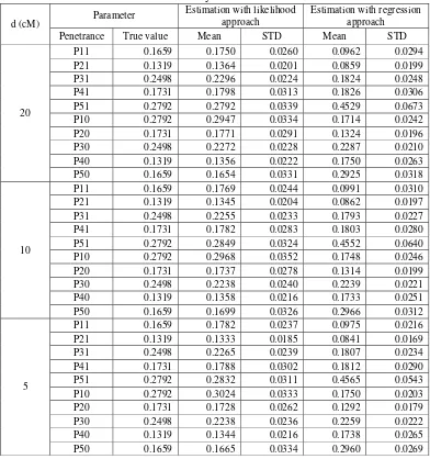
categorize method for ordinal trait... 43 27. Comparison of penetrance estimation using ML and REG approach
under various level of marker distance for binary trait... 48 28. Comparison of penetrance estimation using ML and REG approach
under various level of QTL effect for binary trait ... 48 29. Comparison of penetrance estimation using ML and REG approach for
various shapes of phenotypic distribution for binary trait ... 49 30. Comparison of penetrance estimation using ML and REG approach
under various sample size for binary trait... 49 31. Comparison of penetrance estimation using ML and REG approach
under various level of marker density for ordinal trait ... 50 32. Comparison of penetrance estimation using ML and REG approach
under various level of QTL effect for ordinal trait ... 51 33. Comparison of penetrance estimation using ML and REG approach
under various sample size for ordinal trait... 52 34. Comparison of penetrance estimation using ML and REG approach for
various shapes of phenotypic distribution for ordinal trait ... 53 35. Comparison of penetrance estimation using ML and REG approach
LIST OF FIGURES
Page 1. Conventionally defined backcross progeny for a QTL and two flanking
markers... 5 2. Linkage relationship of a QTL and two flanking markers... 5 3. Liability and threshold model for binary trait... 6 4. Liability and threshold model for ordinal trait... 11 5. Empirical distribution of test statistic under null hypothesis for ML
approach and REG approach for binary trait ... 22 6. Empirical distribution of test statistic under null hypothesis for ML
INTRODUCTION
Background
Genes or loci on chromosome underlying a quantitative trait are called Quantitative Trait Loci (QTL). Many such traits are both important economically as well as biologically such as milk, meat or crop production. Hence, characterizing genes controlling quantitative trait on their position in chromosome and their effect on trait through a process called QTL mapping are needed. The QTL genotypes are unobserved. In addition, the environment also affects the trait making the characterization of QTL become complex.
The idea in locating QTL is if there is association among trait and DNA markers, then the QTL should located near the DNA markers. The statistical method in utilizing this association can be traced back in 1923 when Sax evaluating the association between seed weight as trait of interest and seed coat color as marker and concluded that there is association among them. The method proposed by Sax (1923) then called single marker analysis because it utilizes association between trait and single marker at a time. There are various statistical methods employed in single marker analysis such as T-Test, ANOVA, Linear regression, as well as Likelihood Ratio Test where the hypothesis to be tested is the equality of trait mean among marker genotypes. Single marker analysis is relatively easy to implement, however, the position and effect of QTL are confounded.
To overcome the drawback of single marker analysis, Lander and Botstein (1989) proposed a new method called interval mapping. Its name comes from the idea of this method in locating QTL position. This method evaluating the existence of QTL on certain interval in chromosome flanked by two adjacent markers rather than near certain marker as in single marker. However, the number of QTL could not be determined by this method and the position as well as the effect of QTL could be affected by another QTL located in another interval. Hence, Jansen and Stam (1994) and Zeng (1994) proposed composite interval mapping as extension of interval mapping by incorporating another marker as cofactor.
categorical scale, such as resistance from certain disease. If the resistance from the disease is obtained as suscept or resistance, then the trait is in binary scale, whether if the resistance scored on ordered scale varying from unaffected to dead then the trait is in ordinal scale. Another trait could also be obtained in nominal scale such as shapes and colors of flowers, fruits, and seeds in plants, as well as coat colors. From a theoretical point of view, QTL mapping method assuming continuous trait could not be applied to categorical trait.
In dealing with binary trait, Xu and Atchley (1996) proposed likelihood based method by assuming there is continuous distribution called liability underlying binary trait by means of threshold model. Similar approach proposed by Hackett and Weller (1995) in dealing with ordinal trait. On the other hand, Hayashi and Awata (2006) proposed likelihood based approach in analyzing trait in nominal scale.
Problems
In dealing with QTL mapping for categorical trait, there are several issues occur such as the design of the population, the statistical method employed, the critical value in testing the existence of QTL, the estimate of the QTL effect and location, and missing value in QTL data. Some issues are briefly discussed below.
The design of the population
There are two population types in QTL mapping which are designed and not designed population. The population type determines the statistical method involved in the QTL mapping. Recently, the development of statistical method mainly focuses on designed population. Hence, the development of statistical method on not designed population is needed.
The statistical method employed
QTL effect is replacing by their expected value conditional on the two markers flanked the interval. However, the regression approach in the case of categorical scales is not yet developed.
The critical value in testing the existence of QTL
In characterizing QTL, the analysis is performed by searching or scanning and conducting test at every point on the genome (genome scan) simultaneously. In dealing with simultaneous multiple test such as in genome scan, there are two types of error regarded, which are: comparison-wise error rate and family-wise error rate. Regarding the issue of determining critical value which controlled family-wise error rate in genome scan, Lander and Botstein (1989) (denoted as LB method) and Piepho (2001) (denoted as Piepho method) has proposed their approaches which fast in computation but proposed in the context of QTL mapping for continuous trait. However, their approaches were focused on the test statistic not on the trait data itself. Hence, their approaches are potential to be used in categorical trait. For that reason, the performance of these two approaches is interesting to be explored in categorical trait.
The estimate of the QTL effect and location
quantitative trait. Hence, the development and evaluation of interval estimation in categorical trait is needed.
Missing value in QTL data
Missing data are common in QTL analysis. Common treatment in analysis dealing with missing value is to delete the observation containing missing value. However, ignoring such missing data may result in biased estimates of the QTL effect. Dealing with missing value, Niu et al (2005) proposed EM based Likelihood Ratio Test for handling missing data. This approach is implemented in quantitative trait and the extension on categorical trait is needed.
Objectives
Regarding the issues mentioned above, this research will focus on the second and third issue. The objectives of this research are:
1. Evaluate the performance of likelihood and regression approach in QTL mapping for binary and ordinal trait.
2. Evaluate the performance of LB and Piepho method in constructing critical value in testing the existence of QTL for binary and ordinal trait.
THEORY AND METHODS
Backcross population
In a classical backcross design, the population is generated by a heterozygous F1 backcrossed to one of the homozygous parents (for example, a cross of AaQqBb x AAQQBB)(see Figure 1). The rationale behind the interval mapping can be explained using co-segregation listed in the Table 1 (Liu, 1998). Here, r is recombination rate between marker A and B, whether r1 and r2 is recombination rate
between marker A and QTL Q and QTL Q and marker B, respectively (Figure 2). Recombination rate is defined as ratio between recombinant progeny (progeny which is not parental type, created because of crossover process among homologs during meiosis process) and total progeny. In addition, it is assumed that there is no double crossover between markers.
As mentioned above, the QTL genotypes are unobservable, but the probability of QTL genotypes could be obtained using the information from flanking markers genotypes as listed in Table 1.
AAQQBB X aaqqbb
Parent 1 Parent 2
AaQqBb X AAQQBB F1 Parent 1
AAQQBB, AaQqBb 0.5 (1-r)
AAQqBb, AaQQBB 0.5 r1
AAQQBb, AaQqBB 0.5 r2
AAQqBB, AaQQBb 0
Figure 1. Conventionally defined backcross progeny for a QTL and two flanking markers.
Figure 2. Linkage relationship of a QTL and two flanking markers Expected Frequency
A B
r
Q
r1 r2
(marker) (marker)
Table 1. Co-segregation pattern for backcross design in interval mapping QTL Genotype
Marker Genotype
Observed
Count Frequency
QQ Qq
Expected Value (gi)
Joint frequency
AABB n1 0.5(1-r) 0.5(1-r) 0
AABb n2 0.5r 0.5r2 0.5r1
AaBB n3 0.5r 0.5r1 0.5r2
AaBb n4 0.5(1-r) 0 0.5(1-r)
Conditional frequency
AABB n1 0.5(1-r) 1 0 μ1
AABb n2 0.5r r2/r = 1-ρ r1/r = ρ (1-ρ)μ1 + ρμ2
AaBB n3 0.5r r1/r = ρ r2/r = 1-ρ ρμ1 + (1-ρ)μ2
AaBb n4 0.5(1-r) 0 1 μ2
Mean 0.25 μ1 μ2 0.5(μ1+μ2)
Trait in Binary Scale Threshold model and liability
In dealing with binary trait, it is assumed that there is continuous distribution, say U, underlying binary trait, say Y, referred to as liability (Xu and Atchley, 1996). In relation between liability and binary trait (such as resistance to certain disease), it is assumed that there is threshold (γ) in the scale of liability, below which the individual has unaffected phenotype, and above which it is affected (see Figure 3).
The relation can be summarized by ⎩ ⎨ ⎧ < ≥ = γ u ; γ u ; y i i
i 0 if
if 1
(1)
Maximum likelihood (ML) approach
Using liability model, the one-QTL ML mapping model for a backcross population can be written as
ui = μ + bxi* + εi, i = 1, 2, …, n (2)
where ui is the liability value for individual i, μ is the mean, b is the effect of QTL Q,
xi* taking the value of 1 (0) for homozygote QQ (heterozygote Qq), denotes the
genotypes of Q, εi is environmental deviation and is assumed to follow N(0, σ2).
Since the liability is unobserved, the mean μ and variance of ε can be set at any arbitrary value (for simplicity, it is determined that μ = 0 and σ2 = 1).
Based on the conditional probability of ui given xi*, the conditional
probability of yi given xi* is obtained by
∫
∞ = = γ * i i * i i * ii |x ) f(u|x )d(u|x )
P(y 1
(
γ bx) (
Φbx γ)
Φ
) |x )d(u |x
f(u *i
γ * i * i i * i
i = − − = −
−
=
∫
∞ −
1
1 (3)
where Φ(ξ) stands for the standardized cumulative normal distribution function and ξ is the argument. Analysis involving Φ(ξ) is referred to as probit analysis. However, the probit model is difficult to manipulate because numerical integration is required although the parameters are easy to interpret. So, a logistic model is employed to approximate Φ(ξ) for estimation purpose and is expressed by
) exp( 1 ) exp( ) ( ξ ξ ξ ψ +
= (4)
The relationship between a probit model and a logistic model is Φ(ξ) ≈ψ(dξ), where d = π/√3. Therefore,
)} ( exp{ 1 )} ( exp{ 1 γ bx d γ bx d ) |x P(y * i * i * i i − + − ≈
Since the QTL genotype xi* could be homozygote (1) or heterozygote (0) for
an individual, the likelihood is then a mixture distribution with mixing proportions equivalent to the conditional probabilities of QTL genotypes given two flanking markers, qi1 and qi2 for the QTL genotypes QQ and Qq respectively (see Table 1).
For n individuals in the sample, the likelihood function is
∏ ∑
= = − − = n i j y ij y ijijp i p i
q L 1 2 1 1 ] ) 1 ( [
where pi1 and pi2 denotes the conditional probability of yi = 1 given the QTL
genotypes xi* = 1 and xi* = 0, respectively. The log likelihood function is
∑
∑
= = − − = n i j y ij y ijijp i p i
q l 1 2 1 1 ) ) 1 (
log( . (6)
The first partial derivatives are
∑
= − =
∂
∂ n
i i i i
p y b l 1 1 ) (
ω (7)
and
∑
= − + − − = ∂ ∂ ni i i i i i i
p y p
y l
1 1 0
)] )( 1 ( ) ( [ω ω
γ (8)
where
∑
= − − − − = 2 1 1 1 1 1 1 ) 1 ( ) 1 ( j y ij y ij ij y i y i i i i i i i p p q p p qω . (9)
is the posterior probability of xi* = 1.
By treating ωi as constants, the second partial derivatives are
∑
= − − = ∂ ∂ ni i i i
p p b l 1 1 1 2 2 ) 1 (
ω (10)
∑
= − − = ∂ ∂ ∂ n i i iip p
b l 1 1 1 2 ) 1 ( ω
γ (11)
and ] ) 1 ( ) 1 ( ) 1 ( [ 1 0 0 1 1 2 2
∑
= − + − − − = ∂ ∂ ni i i i i i i
p p p p l ω ω
γ . (12)
simple compared to incomplete data (Pawitan, 2001). In QTL mapping, the unobserved QTL genotype xi* treated as missing data. The EM steps are as follows:
1. Set up initial values of b and γ. Usually b is set to 0, whether γ is set to Σiyi/n
2. Calculate ωi (E-Step)
3. Given ωi, solve for b and γ using the Newton-Raphson iteration (M-Step) as
follow. Let g denote the vector of first partial derivatives and H be a matrix of second partial derivatives. If θ(t) is a vector of solutions at the tth step, the solutions at the (t+1) step is
θ(t+1) = θ(t) + H-1g
4. Update the initial values and go to step 2
5. Repeat steps 2-4 until convergence. Given two convergence criteria εk>0 and
εp>0, the iteration is considered to be converged if one of the following
criteria are satisfied:
a. l(γ(t+1),b(t+1))−l(γ(t),b(t)) <εk b. max
(
γ(t+1) −γ(t),b(t+1) −b(t))
<εpRegression (REG) approach
Using liability model, the one-QTL REG mapping model for a backcross population can be written as
ui = μ + bπi + εi, i = 1, 2, …, n (13)
where ui, μ, b, and εi have the same definitions as in model (2), and πi is the
conditional expectation of QTL genotypes given the two flanking markers. The likelihood function is
∏
=
− − = n
i
y i y
i i p i
p L
1
1
) 1 (
where pi denotes the conditional probability of yi = 1 given the πi. The log likelihood
function is
∑
= + − −
= n
i i i i i
p y p
y l
1
)] 1 )( 1 ( log
The first partial derivatives are
∑
= − = ∂ ∂ ni i i i
p y b l 1 ) (
π (15)
and
∑
= − = ∂ ∂ ni i i
p y l 1 ) (
γ . (16)
The second partial derivatives are
∑
= − − = ∂ ∂ ni i i i
p p b l 1 2 2 2 ) 1 ( π (17)
∑
= − − = ∂ ∂ ∂ n i i iip p
b l 1 2 ) 1 ( π γ (18) and
∑
= − − = ∂ ∂ ni i i
p p l 1 2 2 ) 1 (
γ (19)
The procedure in obtaining parameter estimates are as follow. Let g denote the vector of first partial derivatives and H be a matrix of second partial derivatives. If θ(t) is a vector of solutions at the tth step, the solutions at the (t+1) step is
θ(t+1) = θ(t) + H-1g
The procedure in choosing initial value for γ and b is similar to the procedure in ML approach as mentioned above.
Trait in Ordinal Scale Threshold model and liability
Let U denote the liability underlying ordinal trait Y with c categories. A set of fixed thresholds, γ1, γ2, …, γc-1, on the underlying scale defined the observed
categories on ordinal scale 1, 2, …, c. We thus have model γj-1 < ui≤γj⇔ Yi=j; γ0=-∞; γc=∞
Figure 4. Liability and threshold model for ordinal trait
ML approach
Let the c ordered categories have cumulative probabilities γ1(x*), γ2(x*), ..,
γc(x*), where γc(x*)=1. Then
) bx exp( 1 ) bx exp( ) P(U j) P(Y * j * j j j − + − = ≤ = ≤ = γ γ γ
φ (20)
We can rewrite this as a generalized linear model with logit link function
*
1
log j i
j j
ij ⎟⎟= −bx
⎠ ⎞ ⎜ ⎜ ⎝ ⎛ − = γ φ φ
η (21)
Similar to binary trait, since the QTL genotype xi* could be homozygote (1)
or heterozygote (0) for an individual, the likelihood is then a mixture distribution with mixing proportions equivalent to the conditional probabilities of QTL genotypes given two flanking markers, qi1 and qi2 for the QTL genotypes QQ and Qq
respectively (see Table 1). Let φj1 and φj2 denote the conditional cumulative
probability of yi ≤ j given the QTL genotypes xi* = 1 and xi* = 0, respectively. In
addition, let Rij = Σjzij where zij = 1 if yi = j and j = 1,2, …, c, and
⎟ ⎟ ⎠ ⎞ ⎜ ⎜ ⎝ ⎛ − =
+ k ijk j
i ijk
ijk φ φ
φ ϕ ) 1 ( log
For n individuals in the sample, the likelihood function is
∏ ∑
∏
= = − = − + + + ⎥⎥ ⎥ ⎦ ⎤ ⎢ ⎢ ⎢ ⎣ ⎡ ⎪⎭ ⎪ ⎬ ⎫ ⎪⎩ ⎪ ⎨ ⎧ ⎟ ⎟ ⎠ ⎞ ⎜ ⎜ ⎝ ⎛ − ⎟ ⎟ ⎠ ⎞ ⎜ ⎜ ⎝ ⎛ = + n i k c j R R k j jk k j R k j jk ik ij j i ij q L 1 2 1 11 ( 1)
The log likelihood function is
∑
∑
∏
= = − = − + + + ⎥⎥ ⎥ ⎦ ⎤ ⎢ ⎢ ⎢ ⎣ ⎡ ⎪⎭ ⎪ ⎬ ⎫ ⎪⎩ ⎪ ⎨ ⎧ ⎟ ⎟ ⎠ ⎞ ⎜ ⎜ ⎝ ⎛ − ⎟ ⎟ ⎠ ⎞ ⎜ ⎜ ⎝ ⎛ = + n i k c j R R k j jk k j R k j jk ik ij j i ij q l 1 2 1 11 ( 1)
) 1 ( ) 1 ( ) 1 ( log φ φ φ φ φ . (22)
The first partial derivatives are
∑ ∑
∑
= = − = ∂ ∂ = ∂ ∂ n i k c j ijkt ijk ijk i ik t Q U l l 1 2 1 1 1 ϕ ωθ , (23)
where θt is the t-th parameter of the model (21), and t=1, 2, …, c. In addition,
k j i ijk j i ij ijk
i R R
l ) 1 ( ) 1 ( + + − = ∂ ∂ φ φ
ϕ , (24)
) ( ( 1)
) 1 ( ijk k j i ijk k j i ijk U φ φ φ φ − = + +
, (25)
and k j i k j i k j i ijk t j i ijk ijk ijt
ijkt P P
Q ) 1 ( ) 1 ( ) 1 ( ) 1 ( + + + + ∂ ∂ − ∂ ∂ = η φ φ φ η φ
, (26)
in which ⎪⎩ ⎪ ⎨ ⎧ = − − ≤ ≤ = ∂ ∂ = −
− t c
x c t P c t i jt t ij
ijt ;if
1 1 if ; * )] 1 ( [ δ θ η
δjt = 1 if j=t, 0 otherwise, and Pict=0. For i=1, 2, …, n; j=1, 2, …, c-1,
) 1 ( ijk
ijk ijk
ijk φ φ
η φ − = ∂ ∂
and ∂φict/∂ηict = 0. In addition,
∑
∏
∏
= − = − + + + − = − + + + ⎪⎭ ⎪ ⎬ ⎫ ⎪⎩ ⎪ ⎨ ⎧ ⎟ ⎟ ⎠ ⎞ ⎜ ⎜ ⎝ ⎛ − ⎟ ⎟ ⎠ ⎞ ⎜ ⎜ ⎝ ⎛ ⎪⎭ ⎪ ⎬ ⎫ ⎪⎩ ⎪ ⎨ ⎧ ⎟ ⎟ ⎠ ⎞ ⎜ ⎜ ⎝ ⎛ − ⎟ ⎟ ⎠ ⎞ ⎜ ⎜ ⎝ ⎛ = + + 2 1 11 ( 1)
) 1 ( ) 1 ( 1
1 ( 1)
) 1 ( ) 1 ( ) 1 ( ) 1 ( k c j R R k j jk k j R k j jk ik c j R R k j jk k j R k j jk ik ik j j j j j j q q φ φ φ φ φ φ φ φ φ φ
ω (27)
is the posterior probability of xi*=1 and xi*=0 for k=1 and k=2, respectively. The
second partial derivatives are
∑ ∑
∑
= = − = − = ∂ ∂ ∂ n i k c j ijks ijkt ijk ik s t Q Q U q l 1 2 1 1 1 2 θThe EM steps to obtain parameter estimate are similar as mentioned in binary trait above. In addition, the initial value for b is usually set to 0, whereas for thresholds, the initial values are
⎟ ⎟ ⎠ ⎞ ⎜ ⎜ ⎝ ⎛ − = j j j A A 1 log ) 0 ( γ where n z A n i j m im j
∑∑
= = 1and j=1, 2, …, c-1. On the other hand, the two convergence criteria are as follow: (a) l(γ1(t+1),γ2(t+1),...,γc(t−+11)b(t+1))−l(γ1(t),γ2(t),...,γc(−t)1,b(t)) <εk
(b) max
(
γ1(t+1) −γ1(t),γ2(t+1) −γ2(t),...,γc(t−+11) −γc(t−)1,b(t+1) −b(t))
<εpREG approach
The generalized linear model with logit link function for one-QTL model is
i j j j
ij φ γ bπ
φ η ⎟⎟= − ⎠ ⎞ ⎜ ⎜ ⎝ ⎛ − = 1
log (29)
Let φj denote the conditional cumulative probability of yi ≤ j given the πi. In
addition, let Rij = Σjzij where zij = 1 if yi = j and j = 1,2, …, c. For n individuals in the
sample, the likelihood function is
∏ ∏
= − = − + + + ⎪⎭ ⎪ ⎬ ⎫ ⎪⎩ ⎪ ⎨ ⎧ ⎟ ⎟ ⎠ ⎞ ⎜ ⎜ ⎝ ⎛ − ⎟ ⎟ ⎠ ⎞ ⎜ ⎜ ⎝ ⎛ = + n i c j R R j j j R j j ij j i ij L 1 11 ( 1)
) 1 ( ) 1 ( ) 1 ( φ φ φ φ φ
The log likelihood function is
{
}
∑
∑
= − = − + = n i cj ij ij i j ij
g R R l 1 1
1 ( 1)
) (
log ϕ ϕ (30)
where ⎟ ⎟ ⎠ ⎞ ⎜ ⎜ ⎝ ⎛ − = + ij j i ij
ij φ φ
⎟ ⎟ ⎠ ⎞ ⎜ ⎜ ⎝ ⎛ − = + = + + ij j i j i ij ij g φ φ φ ϕ ϕ ) 1 ( ) 1 ( log )) exp( 1 log( ) (
The first partial derivatives are
∑ ∑
= − =∂ ∂ = ∂ ∂ n i cj ij ij ijt
i t Q U l l 1 1 1 ϕ
θ , (31)
where θt is the t-th parameter of the model (29), and t=1, 2, …, c. In addition,
) 1 ( ) 1 ( + + − = ∂ ∂ j i ij j i ij ij
i R R
l
φ φ
ϕ , (32)
) ( ( 1)
) 1 ( ij j i ij j i ij U φ φ φ φ − = + +
, (33)
and ) 1 ( ) 1 ( ) 1 ( ) 1 ( + + + + ∂ ∂ − ∂ ∂ = j i j i j i ij t j i ij ij ijt
ijt P P
Q η φ φ φ η φ
, (34)
in which ⎪⎩ ⎪ ⎨ ⎧ = − − ≤ ≤ = ∂ ∂ = −
− t c
x c t P c t i jt t ij
ijt ;if
1 1 if ; * )] 1 ( [ δ θ η
δjt = 1 if j=t, 0 otherwise, and Pict=0. For i=1, 2, …, n, j=1, 2, …, c-1,
) 1 ( ij
ij ij
ij φ φ
η φ − = ∂ ∂
and ∂φict/∂ηict = 0. The second partial derivatives are
∑ ∑
= − = − = ∂ ∂ ∂ n i cj ij ijt ijs s t Q Q U l 1 1 1 2 θ
θ (35)
Critical Value
Suppose when we conducted QTL analysis at a certain point in the genome, we determine the type I error of the test equal to α. This kind of error is called comparison-wise error rate (CWER). However, in characterizing QTL, the analysis is performed by searching or scanning and conducting test at every point on the genome (genome scan) simultaneously. Then, the type I error of all the tests simultaneously is larger than α (This type I error related with genome scan simultaneously is called family-wise error rate/FWER). Hence, in characterizing QTL by genome scan, we are concerned with controlling FWER.
There are several methods proposed in controlling FWER. Lander and Botstein (1989) proposed a method in controlling FWER by determining critical value which considering the size of the genome and the distribution of the trait. Consider an organism with C chromosomes and genetic length G, measured in Morgans. When no QTLs are present, the probability that the test statistic exceeds a high level T is ≈(C+2Gt)χ2(t), where t = (2 log 10)T and χ2
(t) denotes the cumulative distribution function of the χ2 distribution with 1 df. In order to make the probability less than α that a false positive occurs somewhere in the genome, the appropriate LOD threshold is thus ≈ Tα = (2 log l0)tα, where tα solves the equation α = (C + 2G tα)χ2(tα) (Lander and Botstein (1989).
On the other hand, Piepho (2001) also proposed method in determining critical value which controlled FWER. He mentioned that for a given critical value T, the upper bound of the FWER is estimated by
⎟ ⎠ ⎞ ⎜ ⎝ ⎛ Γ ⎟
⎠ ⎞ ⎜ ⎝ ⎛− +
>
= − −
k T
VT T
P k k k
2 1 / 2 2 1 exp )
(χ2 (1/2)( 1) (1/2) α
where P(χk2>T) is the cumulative distribution function of χ2 with k df and Γ(.) is the
Gamma function. In addition,
∑
= −
− = P
i
i
i T
T V
2
1)
( )
(θ θ
where T(θ) is the test statistic at the putative QTL position θ in centimorgans and P is the number of putative QTL position evaluated.
method. The idea in permutation test was we develop the empirical distribution of the test statistic, by resampling the original data many times, perform the QTL analysis and record the value of the test statistic obtained at each resampling process. These records of the test statistic are performing as empirical distribution of the test statistic.
Heritability
Dealing with inheritance, there is a concept called heritability (denoted as h2) which is a proportion of genetic variance relative to phenotypic variance. In categorical trait, the liability variance performed as phenotypic variance, where σu2 =
σb2 + σε2. Here, σu2, σb2, σε2 is liability variance, QTL or genetic variance, and
environmental variance, respectively. Hence, heritability is computed as h2=σb2/(σb2+σε2). By definition of QTL genotype (1 for QQ and 0 for Qq as
mentioned above), the liability variance is σu2 = b2/4 + 1 because the environmental
MATERIAL AND METHOD
To assess the performance of ML and REG approach as well as the performance of LB and Piepho method in determining critical value in QTL mapping for binary and ordinal trait, simulation study was conducted. The explanation of the simulation study is as follow.
Design of simulation experiments in evaluation of the performance of ML and REG approach
In evaluation of the performance of the ML and REG approach dealing with binary and ordinal trait, the simulation study was conducted by taking into account several factors that may affecting the performance of the two approaches. The factors are:
a. QTL effect
This factor was used to evaluate whether the statistical method perform better as the QTL more affecting the trait.
b. Number of categories
This factor was evaluated due to in scoring the phenotypic of the trait, the different scoring method as well as the nature of the trait may result in different number of categories. Hence, the effect of number of categories on the performance of statistical method employed is needed to be evaluated. c. Shape of the phenotypic distribution
Similar to number of categories factor, different scoring method as well as the nature of the trait may also result in different shape of phenotypic distribution. Therefore, the effect of shape of the phenotypic distribution on the performance of statistical method employed is needed to be evaluated. d. Sample size
e. Marker density
In constructing the DNA marker map, different organism or method employed may result map with different marker density. Therefore, the evaluation of the effect of marker density on the performance of statistical employed is interesting.
f. The number of QTL
The phenotypic expression of the trait may affected by several QTLs. Therefore, the effect of number of QTL on the performance of statistical method employed is needed to be evaluated.
In the simulation, a backcross population was generated with sample size or number of progeny equal to n. Except for number of QTL factor, in evaluation for other factors, a single QTL affecting the trait with the effect equal to b was placed at position 25 cM from one end of a chromosome with 100 cM long covered by several evenly spaced markers with the distance d from one another. The value of b was chosen such that the heritability h2 will equal to certain value. Moreover, all the settings in the simulation were replicated 200 times. The explanation of the design in the simulation experiments is as follow.
Design of simulation experiments for binary trait
For binary trait, the effect of five factors was evaluated on the performance of likelihood and regression approach. The factors are: (1) QTL effect; (2) shape of the phenotypic distribution; (3) sample size; (4) marker density; and (5) number of QTL.
Evaluation of QTL effect
In the evaluation of QTL effect, the QTL effect was set to four levels, which were, b = 0.4588, 0.6667, 1.0000, 1.6330, so that the corresponding heritability at the four levels are h2 = 0.05, 0.10, 0.20, 0.40, respectively. In this configuration, the ratio of the two categories frequencies was set to 1:1, n = 200, and d = 10 cM.
Evaluation of the shape of the phenotypic distribution
(n=200), a given QTL effect (b=0.6667, that is, h2=0.10), and a given distance among markers (d=10 cM). In this evaluation, the threshold was chosen so that the phenotypic frequency ratio was 1:1 for first set, and 7:3 for second set.
Evaluation of sample size
To evaluate the effect of sample size, four levels of sample sizes was investigated, which were, n=100, 200, 300, 500. In this evaluation, the QTL effect was set to b=0.6667 (corresponds to h2=0.10), d = 10 cM, and the ratio of the two categories frequencies was set to 1:1.
Evaluation of marker density
The simulation experiment intends to evaluate the effect of marker density was performed by setting the value of QTL effect b=0.6667 (corresponds to h2=0.10), under a fixed sample size n=200, and the ratio of the two categories frequencies was set to 1:1. Here, the marker density, d, was set to three levels d=5, 10, 20 cM.
Evaluation of number of QTL
set to 1 if the sum of this value across the three QTLs is at least 2, and set to 0 otherwise.
Design of simulation experiments for ordinal trait
For ordinal trait, the effect of six factors was evaluated on the performance of likelihood and regression approach. The factors are: (1) QTL effect; (2) shape of the phenotypic distribution; (3) sample size; (4) marker density; (5) number of categories; and (6) number of QTL.
Evaluation of QTL effect
The configuration in this evaluation was similar to the binary trait except that the number of phenotypic categories, c was set to 5 with the ratio of the frequency of the categories was set to 1:2:4:2:1.
Evaluation of the shape of the phenotypic distribution
In this design, the number of categories, c, was set to 5. There were three phenotypic frequency ratios to be investigated, that is, 1:1:1:1:1 (corresponds to uniform distribution), 1:2:4:2:1 (corresponds to symmetrical and bell-shaped distribution), and 6:4:3:1:1 (corresponds to skewed distribution). The level of the other factor was similar to the binary trait as mentioned above.
Evaluation of sample size
The evaluation of sample size was conducted similar to binary trait, that was, by set the level of sample size as n=100, 200, 300, 500. The level for other factors are the same as in binary trait except that the number of phenotypic categories was set to 5 and the ratio of the frequency of the categories was 1:2:4:2:1.
Evaluation of marker density
number of phenotypic categories was set to 5 and the ratio of the frequency of the categories is 1:2:4:2:1.
Evaluation of number of categories
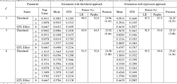
Here, three levels of number of categories, c=3, 5, 8 will be investigated with the phenotypic frequency ratios were set to 1:2:1, 1:2:4:2:1, 1:2:3:4:4:3:2:1, respectively. The QTL effect was set to b=0.6667 (corresponds to h2=0.10), sample size n=200, and marker density d=10 cM.
Evaluation of number of QTL
Evaluation of number of QTL for ordinal trait was similar to ones conducted for binary trait. However, here number of phenotypic categories, c is set to 5 with the ratio of the frequency of the categories was set to 1:2:4:2:1 for first and second setting when the QTLs affecting the trait through threshold model. For the third setting, after give value for each QTL genotype, the observed ordinal trait was set to 1 if the sum of the value across the three QTLs was 0, set to 3 if the sum was 3, and set to 2 otherwise.
Design of simulation experiments for evaluating critical value
RESULT AND DISCUSSION
Result
In this section, the result from simulation experiments for evaluating method in determining critical value will be outlined first. In the next subsection, the result from simulation experiment for evaluating the effect of various factors on performance of ML and REG approach will be outlined started from binary trait to ordinal trait.
Evaluation of methods in determining critical value Result for binary trait
In the evaluation for binary trait, the empirical distribution of test statistic under null hypothesis for ML approach is very close to empirical distribution for REG approach (Figure 5). The exploration on percentile of empirical distribution of test statistic for ML and REG approach also yields similar result (see Table 2 for the detail).
Test St at ist ic
Fr
e
q
u
e
n
c
y
21 18 15 12 9 6 3 0 1200
1000
800
600
400
200
0
ML REG Var iab le
Figure 5. Empirical distribution of test statistic under null hypothesis for ML approach and REG approach for binary trait
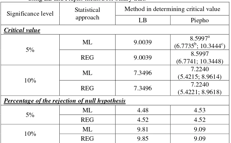
significance level for both approaches, although their average is close to critical value obtained from LB method (see Table 3 for the detail). At 5% significance level, the percentage of the rejection of null hypothesis from 10000 replications in the simulation experiment using critical value obtained from LB method is close to Piepho method (Table 3), whereas at 10% significance level, this percentage from LB method is higher than Piepho method. For both significance levels, the percentages of the rejection of null hypothesis using LB method is close to the significance level, whereas for Piepho method these percentages relatively close only at 5% significance level but not at 10% significance level.
Table 2. Percentile of empirical distribution of test statistic under null hypothesis for ML approach and REG approach for binary trait
No Percentile ML approach REG approach
1 P90 7.3095 7.2937
2 P95 8.8679 8.8697
3 P97.5 10.3296 10.3467
[image:50.612.113.512.426.673.2]4 P99 12.3837 12.3843
Table 3. Critical value and percentage of the rejection of null hypothesis obtained using LB and Piepho method for binary trait.
Method in determining critical value Significance level Statistical
approach LB Piepho
Critical value
ML 9.0039 8.5997
a
(6.7735b; 10.3444c) 5%
REG 9.0039 8.5997
(6.7741; 10.3448)
ML 7.3496 7.2240
(5.4215; 8.9614) 10%
REG 7.3496 7.2240
(5.4221; 8.9618) Percentage of the rejection of null hypothesis
ML 4.48 4.53 5%
REG 4.52 4.52 ML 9.81 9.09 10%
REG 9.85 9.09
Result for ordinal trait
Unlike the result for binary trait, ML and REG approach used in ordinal trait showing different shape of empirical distribution of the test statistic (Figure 6). For this reason, the exploration on the percentiles of empirical distribution of the test statistic for ML approach yield different result with REG approach (Table 4). For example, P90 for empirical distribution of the test statistic of ML approach is 7.2103, whereas for REG approach is 5.8807.
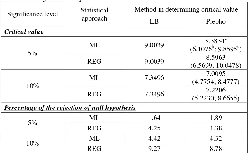
As for binary trait, in determining critical value for ordinal trait, LB method yield single critical value for ML and REG approach, whereas Piepho method yield different critical value which depend on the data used (Table 5). Unlike for binary trait, the average critical value of Piepho method is differ from critical value obtained using LB method for ML approach, whereas for REG approach the average critical value of Piepho method is close to critical value obtained using LB method (Table 5). On the other hand, the percentage of rejection of null hypothesis using LB and Piepho method yield similar result, except at REG approach and 10% significance level where the percentage obtained using Piepho method is lower compare to the percentage obtained using LB method. If we compare the percentage of rejection of null hypothesis obtained using LB and Piepho method with the significance level, these two values are differ significantly for ML approach, whereas for REG approach these two values are only differ slightly (Table 5).
Test St at ist ic
Fr
e
q
u
e
n
c
y
19.25 16.50 13.75 11.00 8.25 5.50 2.75 0.00 700
600
500
400
300
200
100
0
ML REG Var iab le
Table 4. Percentile of empirical distribution of test statistic under null hypothesis for ML approach and REG approach for ordinal trait
No Percentile ML approach REG approach
1 P90 7.2103 5.8807
2 P95 8.6738 7.1038
3 P97.5 10.1720 8.2813
[image:52.612.113.511.232.478.2]4 P99 11.9676 9.9246
Table 5. Critical value and percentage of the rejection of null hypothesis obtained using LB and Piepho method for ordinal trait.
Method in determining critical value Significance level Statistical
approach LB Piepho
Critical value
ML 9.0039 8.3834
a
(6.1076b; 9.8595c) 5%
REG 9.0039 8.5963
(6.5699; 10.0478)
ML 7.3496 7.0095
(4.7754; 8.4777) 10%
REG 7.3496 7.2206
(5.2230; 8.6655) Percentage of the rejection of null hypothesis
ML 1.64 1.89 5%
REG 4.25 4.38 ML 4.42 4.32 10%
REG 9.27 8.78
Note: a, b, c is the average, minimum and maximum critical value obtained using Piepho method
Evaluation of statistical approach in QTL mapping Result for binary trait
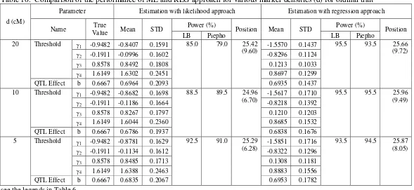
effect, and QTL position tends to close to the true value. Moreover, the statistical power of the ML and REG approach was higher for the denser marker than for the less dense ones.
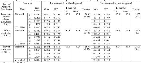
The performance of REG approach was comparable to ML approach in the investigation of the shape of phenotypic distribution (Table 7). As for marker density factor, LB and Piepho method also has similar performance in determining critical value in testing the existence of QTL. In this simulation, it was obtained that the skewed phenotypic distribution has effect in lowering the statistical power for both statistical approaches, especially for REG approach.
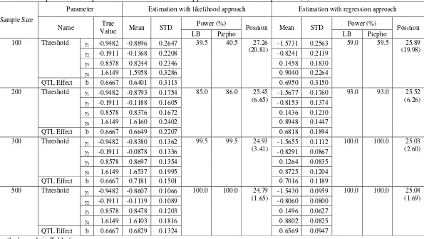
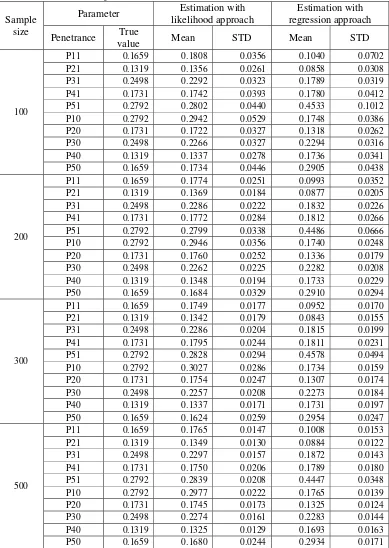
The investigation on effect of sample size factor on the performance of statistical approach yield result that REG approach also has similar performance with ML approach (Table 8). The performance of LB method and Piepho method in determining critical value are also comparable. In addition, the sample size factor affecting the performance of the ML and REG approach on the estimation of threshold and QTL effect, the QTL position as well as the statistical power in detecting QTL. Here, the QTL has higher power to be detected and the threshold, QTL effect, and QTL position were more precisely estimated for larger sample size than for smaller sample size.
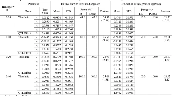
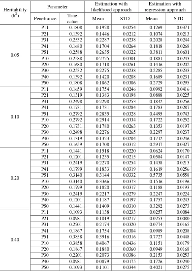
In the evaluation of the effect of QTL effect, the REG approach showing similar performance with ML approach on the estimation of the threshold, QTL effect, QTL position, as well as statistical power in detecting QTL (Table 9). On the other hand, the LB and Piepho method showing similar result in detecting QTL as in the evaluation of the other factors. In addition, the QTL effect factor affecting the performance of the ML and REG approach on the statistical power in detecting QTL as well as the QTL position estimated. Here, QTL with larger effect tends to have a higher power to be detected and the QTL position was more precisely estimated than for smaller one.
56.5% for both approaches if Piepho method was used. However, if we focus on the true position where the three QTLs located ± 10 cM, the ML and REG approach only detect at about 30% for each QTL (Table 10 and Table 11). Moreover, for all of the 200 replications as well as for the replication only when the QTL was detected, the estimation of the QTL effect is far biased to the true QTL effect especially when the REG approach was used.
Another configuration in this simulation when there are more than one QTL affecting the trait through threshold model was QTL had different effect on the trait. In this investigation, the statistical power in detecting any QTL in the two chromosomes was 87.5% and 88.5% for ML and REG approach respectively when LB method used in determining critical value, and 70.5% and 71% for ML and REG approach when Piepho method used. However, the statistical power in detecting each QTL was varied and depended on the QTL effect determined. Here, larger QTL tends to have a higher power to be detected (Table 12 and Table 13). Similar to the configuration of equal QTL effect, in this configuration the estimation of QTL effect was far biased to the true value especially when REG approach was used.
Table 6. Comparison of the performance of ML and REG approach for various marker densities (d) for binary trait
Parameter Estimation with likelihood approach Estimation with regression approach
Power (%)b Power (%)b
d (cM)
Name True
Value Mean STD
a
LB Piepho Position
c
Mean STDa
LB Piepho Position
c
Threshold γ 0.3334 0.3098 0.2697 0.3014 0.2857
20
QTL Effect b 0.6667 0.6148 0.4842
46.0 40.5 33.43
(20.46) 0.6081 0.4909
46.0 40.0 33.36 (20.19)
Threshold γ 0.3334 0.3115 0.2785 0.3058 0.2651
10
QTL Effect b 0.6667 0.6175 0.4802
48.5 50.0 30.66
(23.15) 0.6149 0.4811
48.0 49.5 30.65 (23.13)
Threshold γ 0.3334 0.3374 0.2486 0.3164 0.2380
5
QTL Effect b 0.6667 0.6499 0.4259
52.5 54.5 26.42
(19.56) 0.6556 0.4089
52.0 54.0 26.08 (19.17)
a
STD stands for standard deviation of the estimated parameters obtained from 200 replicated simulations. b
Empirical statistical power was calculated as the proportion of the simulated samples among 200 replicates with the highest test statistical value along the genome greater than the critical value obtained using LB and Piepho method at 5% significant value.
c
The true QTL position is at 25 cM of the simulated chromosome. The standard deviations of the estimated QTL positions (obtained from 200 replicates) are given in parentheses.
Table 7. Comparison of the performance of ML and REG approach for various shapes of phenotypic distribution for binary trait
Parameter Estimation with likelihood approach Estimation with regression approach
Power (%) Power (%)
Phenotypic distribution
Name True
Value Mean STD LB Piepho Position Mean STD LB Piepho Position Threshold γ 0.3334 0.3254 0.1648 0.3361 0.1416
Uniform distribution
(1:1) QTL Effect b 0.6667 0.6277 0.2741
85.5 85.0 26.64 (15.92)
0.6740 0.2214
84.5 86.0 26.49 (11.17)
Threshold γ 0.8578 0.8273 0.1715 0.8149 0.1155 Skewed
distribution
(7:3) QTL Effect b 0.6667 0.6827 0.2699
80.0 78.5 26.35 (11.57)
0.6767 0.1920
75.0 77.5 26.88 (11.05)
Table 8. Comparison of the performance of ML and REG approach for various sample sizes (n) for binary trait
Parameter Estimation with likelihood approach Estimation with regression approach
Power (%) Power (%)
Sample size
Name True
Value Mean STD LB Piepho Position Mean STD LB Piepho Position Threshold γ 0.3334 0.3062 0.2445 0.2975 0.2530
100
QTL Effect b 0.6667 0.6040 0.4482
46.5 48.0 27.86
(22.32) 0.6036 0.4481
47.0 47.5 27.84 (22.31) Threshold γ 0.3334 0.3353 0.1258 0.3222 0.1177
200
QTL Effect b 0.6667 0.6574 0.1695
86.0 86.0 26.27
(11.21) 0.6573 0.1689
86.0 86.0 26.24 (11.22) Threshold γ 0.3334 0.3215 0.0933 0.3289 0.1021
300
QTL Effect b 0.6667 0.6507 0.1488
94.5 95.5 25.28
(5.56) 0.6500 0.1486
94.5 95.5 25.28 (5.57) Threshold γ 0.3334 0.3162 0.0768 0.3167 0.0769
500
QTL Effect b 0.6667 0.6330 0.1138
100.0 100.0 25.13
(1.90) 0.6329 0.1139
100.0 100.0 25.13 (1.95)
see the legends in Table 6
Table 9. Comparison of the performance of ML and REG approach under various levels of QTL effect for binary trait
Parameter Estimation with likelihood approach Estimation with regression approach
Power (%) Power (%)
Heritability
(h2) Name True
Value Mean STD LB Piepho Position Mean STD LB Piepho Position Threshold γ 0.2294 0.2046 0.1814 0.1985 0.1805
0.05
QTL Effect b 0.4588 0.4032 0.3223
38.0 40.0 29.70
(23.68) 0.4030 0.3218
38.0 39.5 29.72 (23.70) Threshold γ 0.3334 0.3207 0.1353 0.3140 0.1305
0.10
QTL Effect b 0.6667 0.6346 0.2047
77.0 78.5 26.47
(9.86) 0.6346 0.2047
77.0 78.5 26.50 (9.86) Threshold γ 0.5000 0.4776 0.1322 0.4708 0.1307
0.20
QTL Effect b 1.0000 0.9480 0.1827
100.0 100.0 24.87
(2.27) 0.9474 0.1818
100.0 100.0 24.87 (2.31) Threshold γ 0.8165 0.7813 0.1632 0.7809 0.1498
0.40
QTL Effect b 1.6330 1.5629 0.2436
100.0 100.0 24.75
(1.38) 1.5633 0.2439
100.0 100.0 24.76 (1.61)
Table 10. ML approach performance for 3 QTLs model with equal QTL effect for binary trait
Parameter Estimate LB Piepho
QTL
Name True
Value Mean
a
STDa Meanb STDb Power
(%)c Mean
b
STDb Power (%)c Effect 0.4588 0.9482 0.2695 1.2025 0.1767 1.2025 0.1767 1st
Position 25 26.0174 3.2421 26.2514 3.2784 29.0
26.2514 3.2784 29.0
Effect 0.4588 1.0643 0.2519 1.2497 0.1829 1.2586 0.1779 2nd
Position 50 49.2419 2.7586 49.5100 2.6030 35.0
49.4953 2.6401 34.0
Effect 0.4588 0.7277 0.5710 1.2092 0.1679 1.2092 0.1679 3rd
Position 30 37.1550 21.2939 31.0778 10.1197 29.5
31.0778 10.1197 29.5
a
Mean and standard deviation (STD) of the estimated parameters was calculated from 200 replicated simulations. b
Mean and STD of the estimated parameters was calculated only from replicated simulations which succeed to detect the respective QTL using critical value obtained using LB and Piepho method at 5% significant value.
b
Empirical statistical power was calculated as the proportion of the simulated samples among 200 replicates with the highest test statistical value along the three genome segments at the true QTL position ± 10cM that greater than t