EVOLUTIONARY DESIGN OF PROCESS CONTROLLERS
DP Searson, MJ Willis and GA Montague
University of Newcastle upon Tyne, England.
The Genetic Programming (GP) architecture offers a potentially powerful framework for ‘intelligent’ controller design due to its inherent matching of structure to utility. This article describes the use of GP to design discrete time single loop controllers for two different processes: a linear Auto-Regressive eXogeneous (ARX) type system and a non-linear simulated Continuous Stirred Tank Reactor (CSTR), both with constraints on the actuator outputs. It is demonstrated that the GP methodology is capable of designing recursive controllers that, for a specific class of control objectives, offer similar performance to PID controllers on the nominal systems. The advantages and disadvantages of controllers designed in this way are also discussed.
INTRODUCTION
One approach in control systems design is to optimise the parameters of a controller of known structure. This can be done using numerical methods, adaptive techniques or manual tuning methods. These systems
are then known as parameter optimised control systems
[Isermann (1)] and a common example of this type of system is the widely known PID controller.
A contrasting approach is the use of structure optimal
control systems in which both the structure and the parameters of the controller are matched in some way to the parameters and structure of the process model [Isermann (1)]. The deadbeat and Dahlin controllers are examples of structure optimal systems. The applicability of these types of controller is quite restricted, however, because processes with non-linearities and constraints generally do not lend themselves to the analytical approach that the structure optimal control design method requires. Another problem is that the designer
must know a priori what form the controller is to take.
Ideally, it would be desirable to have a method that, given a model of the process, could generate a controller without the designer needing to specify beforehand what form it should take. It would also be desirable that this method could be used with non-linear process models of arbitrary structure as well as utilising any additional information that is available about constraints. The advantage of this over parameter optimised controller design would be that no possibly performance-restricting decisions on the controller structure would need to be made, and better closed-loop control could be achieved.
In reality, this is quite a demanding design problem: any form of automated design procedure cannot easily utilise qualitative knowledge about the process that the control engineer normally has access to and must rely on closed-loop simulations to extract ‘knowledge’ about the problem. Additionally, any controllers produced will have no guarantee of good robustness or stability properties unless provision for this is specifically made in the automated design procedure. This, however, would not be easily achievable for controllers of arbitrary structure.
This article does not seek to fully address the latter problem but instead concentrates on the more tractable task of simple step-change servo control for two nominal processes. This is accomplished by utilising the evolutionary computation method called Genetic Programming (GP), which was developed by Koza (2), to evolve the structure and parameters of simple recursive single loop controllers.
The ideas behind GP are first explained and then the control problem formulation, GP configuration and the two example processes are described. Finally, the results are presented and discussed.
INTRODUCTION TO GP
GP is a method of getting computers to learn how to solve problems without being explicitly programmed to do so. Koza (2) popularised the technique and applied it to a number of problems e.g. symbolic regression, and finite state automata. Although most applications of GP are in the field of computing science recently there have been a number of engineering applications.
In the field of control Alba et al. (3) used GP based
fuzzy logic controllers on the cart-centering control problem first tackled using ordinary GP in Koza (2). Howley (4,5) used GP to derive algorithms to perform specific spacecraft attitude manoeuvres and also to derive control laws for a two-link payload manipulator problem. For further details of engineering applications
the survey given in Willis et al. (6) should be referred
to.
Tree structure of GP
Given a problem, GP works by maintaining a population of individuals, each of which is a computer program that can be ‘executed’ to give a potential solution to the problem. These candidate programs are encoded as parse trees (rather than lines of computer code). Figure (1) depicts a simple example of a tree-structured program. The result of the program is always returned at the top of the tree. In the case of Figure (1)
the program result is (3-b)+2.
Each node of the tree is either a terminal node or a
primitive functional node. Terminals are usually specified to be variables (from the problem at hand) that the designer has previously identified to be ‘inputs’ to the problem. However, terminals can also be defined as constants that are generated randomly when initially creating the tree.
Primitive functionals are usually specified to be ‘operators’ that the designer believes will enable a correct solution to be constructed from the terminals. The selection of the appropriate primitive functionals for a problem is, again, a choice that must be made by the designer. A typical primitive functional set would probably include the standard operators of addition, multiplication, division and subtraction as well as any other operators that the designer suspects to be of use in the context of the problem. Koza (2) states that ability of the sets of terminals and primitive functionals to
solve the selected problem is known as the sufficiency
property of the GP and that for certain classes of problems, e.g. Boolean problems, the sufficient primitive functional set is known exactly. As we move towards more complex problems, however, the minimally sufficient requirements for a problem solution become less clear.
In the case of Figure (1) the terminals that have been utilised to construct the tree are the constants 2 and 3
and the variable b. The primitive functionals used are
the scalar operators ‘+’ and ‘-‘. Generally, tree
programs do not need to use all the terminals or primitive functionals available as the GP algorithm assembles them in a probabilistic manner during a run.
+
- 2
b 3
Figure 1: A simple tree-structured program
Basic GP Algorithm
The measure of success of any individual tree program is calculated by use of some performance criterion or
‘fitness function’. The form of the fitness function is dependent on the problem at hand and must be selected by the designer.
The initial population of individual programs is generated randomly from the sets of terminals and primitive functionals. Each of the individual programs is then executed and its fitness (at providing a solution to the designated problem) determined. The most successful individuals are then used as ‘parents’ for a new generation of individuals. These offspring are created using special reproductive operators (crossover, mutation and direct reproduction) that combine parts of the parent programs in such a way as to preserve valid program syntax in the members of the new generation. The probability of selecting each of the reproductive operators is an algorithm control parameter of the GP that must be decided upon by the designer.
The entire process is continued over a number of generations until a pre-defined fitness criterion is reached or until a set number of generations, e.g. 100, has been completed. The final population of solutions can then be inspected manually by the designer for suitability as a problem solution. The method is known as Genetic Programming because much of the process can be explained in terms of an analogy to Darwinian natural selection.
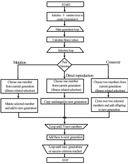
START
Initialise N random trees to create Generation 0
Calculate fitness values Main generation loop
Selection loop
Pick Operator
Direct reproduction
Choose one member from current generation (fitness related selection)
Mutation Crossover
Copy unchanged to next generation Choose one member
from current generation (fitness related selection)
Mutate selected member and add to new generation
Choose two members from current generation (fitness related selection)
Cross over two selected members and add offspring
to new generation
Loop until N new members
Add these to next generation
Loop until max. generations or success criterion reached
STOP
Figure 2: Flowchart of Basic GP procedure
In essence, the mechanism of GP is the random juxtaposition of ‘genes’ from successful parents that
produce offspring that are, on average, fitter than their
simultaneously utilised in a probabilistic manner when producing the search points in the next stage of the process. Another advantage of GP is that the performance criterion need not be continuous and/or differentiable, this means that complex and ‘real-life’ performance measures can be incorporated directly into the GP algorithm. A flowchart of the basic GP procedure is shown in Figure (2).
Reproductive Operators
The primary reproductive operator in the GP algorithm is the crossover operator. The purpose of this is to create two new trees that contain ‘genetic information’ about the problem solution inherited from two ‘successful’ parents. A crossover point (node) is randomly selected in each parent tree. The subtree below this point in the first tree is then swapped with the subtree below the crossover point in the other parent, thus creating two new offspring.
The direct reproduction operator is the simplest of the GP operators, it copies the selected ‘successful’ parent unchanged into the new generation. The purpose of this is to ensure that good genetic material is successfully propagated from one generation to the next whilst avoiding the possible disruptive effects of crossover and mutation.
The mutation operator is used to enhance the diversity of trees in the new generation thus opening up new areas of ‘solution space’ to investigation by the GP. It works by selecting a random crossover point in a single parent and removing the subtree below it. A randomly generated subtree then replaces the removed subtree.
CONTROLLERS AS TREE PROGRAMS
Although the purpose of this work was to generate controllers whose structure was to be optimised to the particular process/performance criteria in question, it was decided that the terminal and primitive functional sets should, as a minimal requirement, be able to easily represent PID controllers. In addition it was decided to force the GP to produce recursive controllers i.e.
controllers whose output, u(k), is equal to the controller
output from the previous time step, u(k-1) plus some
corrective term. The reason that this format was chosen is due to the way of representing the positional form of the discrete PID controller as a tree structured program.
(
)
ss s d k i i s u k e k e T T i e T T k e K k u + − − + + =∑
− = ) 1 ( ) ( ) ( ) ( ) ( 10 (1)
Equation (1) describes a discretised (by rectangular
integration) positional PID controller where uss is the
control signal at the steady state, K is the proportional
gain, e(k) is the setpoint error at time k, Ts is the sample
time (assumed small compared to the dominant time
constant of the process to be controlled), Ti is the
equivalent continuous controller integral time and Td is
the equivalent continuous controller derivative time. If, however, we were to try to represent this as a tree
program using e(k), e(k-1) etc. as terminals then we
would need to define a general purpose integrator as a member of the primitive functional set (one of the restrictions of GP is that any primitive functional must be able to accept any legal subtree, including those containing nested integrators, as an argument). This means that the value of any subtree that should happen to be an argument of the general purpose integrator functional must be stored for each time step in the closed loop simulation. This, in itself, is not a problem
but it was felt that the recursive form of the PID
controller, see Equation (2), could be represented more simply and elegantly as a tree program without recourse to a specific integrator primitive. The recursive form can be generated from Equation (1) by the use of the backward differencing method.
)
2
(
)
1
(
)
(
)
1
(
)
(
k
=
u
k
−
+
q
0e
k
+
q
1e
k
−
+
q
2e
k
−
u
(2)Where:
+
=
s dT
T
K
k
01
(3)
+
−
−
=
i s s dT
T
T
T
K
k
11
2
(4)s d
T
T
K
k
2=
(5)The GP can be forced to produce recursive programs by
fixing the u(k-1) term i.e.
u(k)= u(k-1) + [tree program] (6)
In which case the tree program shown in Figure (3) represents the recursive PID controller of Equation (2)
in a very straightforward manner. The recursive form
has the added of advantage of easy switching between manual and automatic modes during closed loop simulation of the controller/process system.
Of course, it is possible (and desirable) to construct controller trees from richer sets of terminals and functions than utilised in Figure (3). Past process outputs and inputs can also be used as terminals and sigmoidal processing elements (similar to those used in
Artificial Neural Networks) and ‘If-Then-Else’ type
assemble the most appropriate controller structure for a given process model/performance criterion.
q0 e(k) q1 e(k-1) q2 e(k-2)
* * *
+
Figure 3: Tree representation of recursive PID.
CONTROL PROBLEM FORMULATION
The GP was set up to construct a recursive algorithm of the form described by Equation (6). The performance criteria used were based on the transient time responses of the closed loop systems to setpoint step changes. The
closed loop system is simulated over P randomly
generated setpoint changes ∆Sj (j=1,2,3…P). Each
response is run over n discrete time steps. The
performance criterion, I, used for both example
processes is described by Equation (7).
∑ ∑
==
∆
∆
+
=
Pj
j n
k
S
k
u
r
k
e
k
I
1
2
0
(
)
(
)
(7)
This performance criterion seeks to minimise the
setpoint error, e(k), using an Integral of the
Time-weighted Absolute Error (ITAE) term to give increased weighting to steady state errors. It also includes a term,
∆u(k), which describes the control effort exerted since
the previous timestep and is weighted using some
constant r . The resulting value for the response is then
scaled according to the magnitude of the current
setpoint step change ∆Sj. This is done in order to prevent
contributions form the large step changes dominating those form smaller steps when they are finally summed to give I.
The P setpoint changes were generated every at
generation of the GP, rather than using a fixed set throughout. This was done in order to produce controllers that would work well over the entire operating regions of the processes and not just on the specific examples presented during the GP’s ‘training’. Although a performance criteria that is non-stationary from generation to generation is produced, this is not a problem for the GP as the candidate programs selection probabilities are calculated by ranking them relative to each other rather than using absolute fitness values.
DESCRIPTION OF ARX PROCESS
A second order linear process of the form of Equation
(8) was used. The manipulated variable is u(k-1) and the
controlled output is y(k).
)
(
)
1
(
)
(
k
Bu
k
C
k
Ay
=
−
+
ε
(8)A, B and C are polynomials in the backshift operator z-1
and ε(k) is a stationary white noise sequence. In this
case the noise term was set to zero to give a deterministic process.
The process input is constrained at high and low hard limits and also rate-constrained so that it could not change too rapidly from one step to the next. The random setpoint changes presented to the GP were constrained within a pre-defined operating region.
DESCRIPTION OF NON-LINEAR CSTR
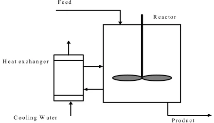
A schematic of the CSTR system is shown in Figure (4).
F e e d
P r o d u c t R e a c to r
H e a t e x c h a n g e r
C o o lin g W a t e r
Figure 4: Schematic of CSTR process.
In this system the objective is to control the reactor temperature with the cooling water to the heat exchanger as the manipulated input.
Reactant A enters the reactor in the feed stream and the exothermic reaction AÆBÆC takes place with B and C as products. The extent of the reaction is dependent on the reactor temperature and so to control the proportions of B and C in the product stream the temperature is manipulated by means of a pump-around heat exchanger.
As for the ARX process, the CSTR system was also made subject to constraints on the manipulated input and, again, the setpoints presented to the GP were fixed to lie within a certain operating region.
fixed step-length using a fourth order Runge-Kutta method.
GP CONFIGURATION
In configuring the GP the population size, reproduction operator selection probabilities, number of fitness cases per generation (i.e. number of setpoint changes) and the total number of generations were decided upon. This was accomplished in an heuristic manner based, in part, on some trial runs and also on values frequently cited in the literature.
Table (1) shows the values of the most important GP algorithm control parameters as well as a summary of the terminal and primitive functional sets used.
Population Size: 200
Termination Criterion: 100 generations elapsed Number of setpoint
changes:
5 per generation Number of time steps per
setpoint change:
ARX: 100 CSTR: 140 Max. allowed program
size:
Approximately 100 nodes Terminals: Current and past two values
of setpoint error, e(k), and output, y(k).
Primitive Functionals: +, -, *, /, exponential function, square root function , natural log function, the backshift operator z-1, the If-Then-Else
operator and a non-linear transfer function.
Table 1: Some GP configuration details
The closed-loop simulation of the systems in response to the setpoint changes is the most CPU intensive part of the GP optimisation process and places a real limit on the number of setpoint change scenarios that may be used in ‘training’ the controllers. For the same reasons it was found to be necessary to limit the size of the controller trees (each of which is executed at every discrete time step of each setpoint change response) in order to keep computing time to a reasonable level. Some of the primitive functionals cited in Table (1) are worthy of further explanation:
The If-Then-Else function compares the values of its first two arguments. If the first is smaller the third argument is executed otherwise the fourth argument is executed.
The backshift operator returns the value of its single argument that was calculated one time-step previously. The use of this operator allows values of errors and outputs further back in time than explicitly presented in the terminal set to be accessed.
The non-linear transfer function is a sigmoidal function whose degree of non-linearity depends on the product of
the two arguments. Sharman et al. (7) used this function
in GP design of signal processing algorithms and Esparcia-Alcazar and Sharman (8) have used it with a GP in evolving the structures of recurrent neural networks.
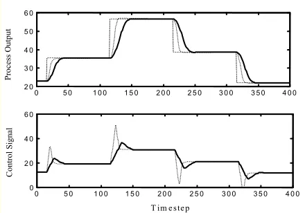
RESULTS
For each process the GP was run approximately 25 times and, after each run, the best of run controllers were extracted and then tested on a number of setpoint changes across the operating regions that were defined during the training process.
For both the CSTR and the ARX systems it was found that approximately one third of the controllers gave unacceptable performances i.e. they became unstable, gave very large steady-state offsets or extremely oscillatory responses to the step changes in setpoint. Another third of the controllers could be simplified to recursive form PID controllers. These gave varying performances depending on the evolved parameter values but they were generally equivalent to those obtained through a trial and error PID tuning exercise. The remaining third of the controllers were not of the PID type and usually included many of the ‘non-linear’ primitive functionals including the non-linear transfer
function and the If-Then-Else operator.
Typical responses for the better GP designed controllers to setpoint step changes are shown in Figure (5) for the ARX process and Figure (6) for the CSTR system. In addition, the manipulated input plots are shown beneath the output responses. In each of these cases, for comparison purposes, the response to the same setpoint changes is shown for a recursive PID controller. These comparison PID controllers were tuned by first using a trial and error method to determine reasonable values of the parameters and then using a Simplex optimisation method to further fine-tune these parameters to the
performance criterion I.
0 5 0 1 0 0 1 5 0 2 0 0 2 5 0 3 0 0 3 5 0 4 0 0 2 0
3 0 4 0 5 0 6 0
0 5 0 1 0 0 1 5 0 2 0 0 2 5 0 3 0 0 3 5 0 4 0 0 0
2 0 4 0 6 0
T im e s te p
Contr
o
l S
ign
al
Pr
oc
ess O
u
tput
Figure (5): ARX system. GP and PID responses Solid Line: GP controller
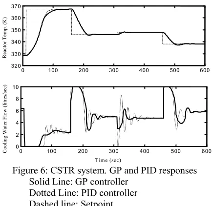
0 100 200 300 400 500 600 320
330 340 350 360 370
0 100 200 300 400 500 600
0 2 4 6 8 10
Tim e (sec)
Cooling Water Flow (l
itres/
sec)
R
ea
ct
o
r
T
em
p
.
(K
)
Figure 6: CSTR system. GP and PID responses Solid Line: GP controller
Dotted Line: PID controller
Dashed line: Setpoint
It can be seen that in both cases the GP controller offers similar performance to the PID controllers. For the ARX system the PID controlled output rises to the setpoint more quickly but in the case of the CSTR system the controlled output plots are virtually identical. In addition to the testing against new step change scenarios the GP and PID comparisons controller were also tested for their performance on disturbance rejection problems for the same systems with load changes applied to the outputs. The PID comparison controllers successfully managed to regulate the processes at steady state but the GP controllers frequently gave very poor responses or became unstable.
The actual structure of the non-linear controller algorithm varies greatly depending on the run and the algorithms themselves are usually very lengthy and difficult to follow. Hence, it does not seem likely that the GP is converging to any particular optimal controller structure. It seems that GP empirically determines a number of solutions for a given problem and there is no real way of analytically determining even simple properties of these solutions without actually executing them as programs.
CONCLUSIONS
It has been demonstrated successfully that Genetic Programming is capable of constructing satisfactory controllers for a specific class of control objectives. By randomly generating the training cases at each generation the controllers have ‘learnt’ to control scenarios they were not explicitly presented with during the training phase. This generalisation property does not always extend to different control objectives, however, when presented load regulation problems the GP controllers tended to fail. It is difficult to analyse the GP designed controller algorithms to see why they do this
because they are not easy to interpret upon inspection and do not appear to have any physical interpretation. Another problem is that at no part of the design process is the stability of the closed-loop system explicitly considered. For example, even with comprehensive post-run testing, there is no guarantee that the controller will work for all step changes presented to them. This would obviously be a major issue in any practical application.
Future work will consider the effect of using a transient response performance envelope based fitness criterion as well as improving the robustness properties of the GP designed algorithms.
BIBLIOGRAPHY
1. Isermann R, 1989, “Digital Control Systems”, Vol.
1, 2nd Edition, Springer-Verlag.
2. Koza J, 1992, “Genetic programming: On the
programming of computers by means of natural selection”, The MIT press.
3. Alba E, Cotta C and Troya J M, 1996,
“Type-constrained Genetic Programming for Rule-Base Definition in Fuzzy Logic Controllers”, GP ‘96-
Proceedings of the 1st Annual Conference, July
28-31, 1996.
4. Howley B, 1996, “Genetic Programming of
Near-Minimum-Time Spacecraft Attitude Maneuvers”,
GP ‘96- Proceedings of the 1st Annual Conference,
July 28-31, 1996.
5. Howley B, 1997, “Genetic Programming and
Parametric Sensitivity: a Case Study in Dynamic Control of a Two-Link Manipulator’, GP ’97- Proceedings of the Second Annual Conference, July 13-16 1997
6. Willis M, Hiden H, Marenbach P and McKay B,
1997, “Genetic Programming: An Introduction and
Survey of Applications”, GALESIA 97 - 2nd
International Conference on Genetic Algorithms in Engineering Systems, September 1-4 1997.
7. Sharman K C, Esparcia-Alcazar A I and Li Y,
1995, “Evolving Signal Processing Algorithms using Genetic Programming”, IEE conference on Genetic Algorithms in Engineering Systems, Conference Number 414, September 12-14 1995.
8. Sharman K C and Esparcia-Alcazar AI, 1997,