Analysis of Variance of Integro-Differential
Equations with Application to Population
Dynamics of Cotton Aphids
Xueying W
ANG, Jiguo C
AO, and Jianhua Z. H
UANGThe population dynamics of cotton aphids is usually described by mechanistic mod-els, in the form of integro-differential equations (IDEs), with the IDE parameters repre-senting some key properties of the dynamics. Investigation of treatment effects on the population dynamics of cotton aphids is a central issue in developing successful chem-ical and biologchem-ical controls for cotton aphids. Motivated by this important agricultural problem, we propose a framework of analysis of variance (ANOVA) of IDEs. The main challenge in estimating the IDE-based ANOVA model is that IDEs usually have no analytic solution, and repeatedly solving IDEs numerically leads to a high computa-tional cost. We propose a penalized spline method in which spline functions are used to estimate the IDE solutions and the penalty function is defined by the IDEs. The esti-mated IDE solutions, as implicit functions of the parameters, are inputs in a nonlinear least squares criterion, which in turn is minimized by a Gauss–Newton algorithm. The proposed method is illustrated using simulation and an observed cotton aphid data set.
Key Words: Cotton aphid; Generalized mechanistic model; Kindlmann–Prajneshu model; Penalized spline.
1. INTRODUCTION
Aphids are small sap sucking insects which can draw a large amount of sap out of plants and make their leaves and stems distorted (Blackman and Eastop2000). Aphids inflict enormous damage on agricultural crops and forest trees (Dixon1998), resulting in worldwide loss of billions of dollars on food and feed grains annually (Metcalf and Metcalf 1995). The primary economic losses caused by aphids take place on wheat, barley, corn,
Xueying Wang is a joint postdoctoral fellow, Applied Mathematics and Computational Science and Department of Mathematics, Texas A&M University, College Station, TX 77843-3143, USA (E-mail:[email protected]). Jiguo Cao (
) is Assistant Professor, Department of Statistics and Actuarial Science, Simon Fraser University, Burnaby, BC, V5A 1S6, Canada (E-mail:[email protected]). Jianhua Z. Huang is Professor, Department of Statistics, Texas A&M University, College Station, TX 77843-3143, USA (E-mail:[email protected]).
© 2013 International Biometric Society
Journal of Agricultural, Biological, and Environmental Statistics, Volume 18, Number 4, Pages 475–491 DOI:10.1007/s13253-013-0135-0
sorghum, oats, and cotton (Tatchell1989). For instance, the cotton aphids, also calledAphis gossypii Glover, are renowned as one of the most devastating pests of US cottons (Leclant and Deguine1994). In 2007, cotton aphids infected about 64 % of US cotton fields, leading to 6.7 million acres of losses of cotton production (Williams2008).
In order to develop successful chemical and biological controls for aphids, the dy-namics of aphid population has to be studied and understood. Since Barlow and Dixon (1980), there has been a considerable number of work to develop mathematical models for quantifying the aphid population dynamics. A cumulative density-dependent mech-anistic model was proposed by Kindlmann (1985) and solved analytically by Prajneshu (1998). This mechanistic model, called the Kindlmann–Prajneshu model (KPM), captures the adverse effect of honeydew accumulation on aphid survival and has gained accep-tance in fitting experimental aphid population data (Kindlmann, Arditi, and Dixon2004; Matis et al.2006,2007a,2007b). Nevertheless, the solution of the KPM model is reflec-tion symmetric and cannot capture the left skewness presented in observed data; see Way (1967), Rabbinge, Ankersmit, and Pak (1979), Mashanova, Gange, and Jansen (2008), and Figure2 of the current paper. To overcome the drawback of KPM, Matis et al. (2007c) proposed a more practical power-law generalization of KPM, called the generalized mech-anistic model (GMM). Although GMM has the desired properties in modeling aphid pop-ulation dynamics, it has not been used to fit experimental data mainly because it has no analytic solution and there is no method available for parameter estimation.
The purpose of this paper is to fill in the gap and develop a penalized spline method for fitting the GMM to the empirical data of cotton aphids. We develop our method in a gen-eral framework where the population dynamics is specified by gengen-eral integro-differential equations (IDEs) for which the GMM is a special case, and the IDE parameters satisfy an analysis of variance (ANOVA) model. The ANOVA model has been widely used in statis-tics to study treatment effects, but its use in the context of IDEs is novel. To address the issue that the IDEs may not have an analytic solution, linear combinations of spline basis functions are used to estimate the IDE solutions and penalty functions defined by the IDEs are employed to ensure the closeness of the spline approximations to the IDE solutions. In our method, the IDE solutions are implicit functions of the IDE parameters and such implicit functions are used in the nonlinear least squares fitting criterion. Our method does not rely on application of numeric IDE solvers, and thus can avoid the potentially high computational cost for repeatedly solving the IDEs.
2. REVIEW OF MECHANISTIC MODELS
LetN (t )denote the aphid population size at timet, andF (t )=0tN (s) dsdenote the cumulative density up to timet. The mechanistic model of Kindlmann (1985) states that
dN (t )
dt =λN (t )−δF (t )N (t ), (1) whereλis the birth rate parameter, andδis the death rate parameter. This model assumes that the growth of aphid population is determined by the net difference between birth rate, λN (t ), and death rate,δF (t )N (t ). The dependence of aphid death rate on the cumulative density is supported by the facts that honeydew excreted by the aphids degrades the living environment of aphids, and the area covered by honeydew is proportional to the cumulative density of the aphid population in the past (Dixon1998). Prajneshu (1998) showed that the analytic solution of (1) takes the form
N (t )=aexp(−bt )1+dexp(−bt )−2. (2) DenoteN0=N (0)andNmaxfor the unique maximum ofN (t ). The three parameters,a, b, andd, in (2) satisfy the following relationships:N0=a/(1+d)2,λ=b(d−1)/(d+1), δ=b2/(2Nmax), andN0=4dNmax/(1+d)2. These relationships can be used to reparam-eterize the analytical solution using interpretable parameters,λ,δ, andNmax. Model (1) is often referred to as the Kindlmann–Prajneshu Model (KPM).
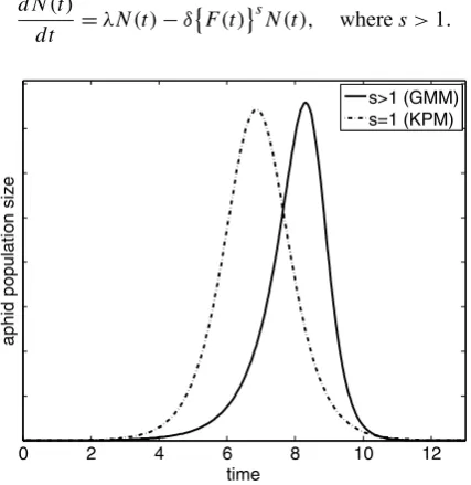
Figure1 shows that the analytic solution of the KPM is reflection symmetric. Using observed data, Matis et al. (2007c) argued that the curve of aphid population size as a function of time should be left-skewed, a feature that the KPM model cannot capture. Therefore, Matis et al. (2007c) suggested the following power-law generalization of the KPM:
dN (t )
dt =λN (t )−δ
F (t )sN (t ), wheres >1. (3)
Equation (3) is referred to as the generalized mechanistic model (GMM). As one can see from Figure1, the solution of the GMM is left-skewed. Whens=1, the GMM is reduced to the KPM, and the corresponding solution is symmetric. Thus, sis a power parameter controlling the skewness of the solution of the GMM.
Figure 1 also shows that, under the GMM, the population gradually grows before achieving its peak value, and then quickly falls down. Thus GMM captures three key fea-tures of the underlying biological principles for aphid population dynamics: (a) offspring production is prolific; (b) growth is constrained by the cumulative density of the past gen-erations; (c) the population diminishes rapidly after the population peak, which is due to the rapid departure of the aphids once their local resources are depleted.
3. APHID EXPERIMENTAL DATA AND THEIR IDE-BASED
ANOVA MODEL
Irrigation water and nitrogen fertilization are two primary factors affecting cotton pro-duction. To investigate the effects of various water and nitrogen treatments on the popula-tion dynamics of the cotton aphids, an experiment was conducted in 2004 at the Texas A&M Agricultural extension center in Lubbock, TX. Three irrigation levels and three nitrogen fertilization treatments are tested in a randomized block split-plot experimental design (Jones and Nachtsheim2009). The three irrigation levels are 65 % (low), 75 % (medium) and 85 % (high), which are indexed asi=1,2,3 in this paper. The three levels of nitrogen treatments are no nitrogen (zero), variable-rate-nitrogen (variable), and blanket-rate-nitrogen (blanket), which are indexed asj =1,2,3. In this design, three blocks are chosen in distinct areas, and they are indexed ask=1,2,3. Within each block, three dif-ferent water treatments are arbitrarily applied to three whole plots. Within each whole plot, three nitrogen treatments are arbitrarily assigned to three split plots. There are a total of 27 experimental units. The number of aphids was counted at seven time points in a nearly weekly pattern between July 26 and September 10 at each experimental unit. More details of the experiment and data can be found in Matis et al. (2008).
Figure2 displays the number of observed cotton aphids over a nearly 7-week period under the blanket-rate-nitrogen treatment. It shows that the data tend to be skewed to the left: the aphid population appears to slowly increase in the first three or four weeks; then the number of cotton aphids exponentially increases until it reaches a peak value in the next two or three weeks; thereafter, the aphid population declines rapidly.
To test the effects of water and nitrogen treatments on the dynamics of the cotton aphid population, Matis et al. (2006,2007a,2007b) performed a two-way analysis of variance (ANOVA) using parameters in the fitted KPM as the response variables. The adoption of the KPM was mainly due to its tractability. However, as shown in Figure2, the solution of the KPM is inconsistent with the skewness of observed data. Since the method that we develop in this paper does not rely on availability of analytical solutions of IDE models, we shall use the more accurate GMM in this paper.
Figure 2. The number of cotton aphids over a nearly 7-week period under the blanket-rate-nitrogen treatment for all combinations of three irrigation levels and the three blocks. The columns correspond to low, medium, and high water treatments from left to right, respectively. The rows correspond to Block 1,2, and 3 from top to bottom, respectively. Thex-axis is the time in weeks. They-axis is the aphid count. The observed data are displayed in circles. The solid and dashed curves are the numeric solutions of the GMM (3) and the KPM (1) using the estimated parameter values.
of aphids at timetij knunder theith level of water treatment and thejth level of nitrogen treatment at thekth block, where i=1,2,3, j =1,2,3, k=1,2,3, andh=1, . . . ,7. BecauseYij knis always positive, it is assumed to follow a log-normal distribution:
log(Yij kn)=log
Nij k(tij kn)
+ǫij kn, (4)
whereNij k(tij kn)is the true aphid population size at timetij kn, andǫij kn’s are independent normally distributed errors with mean 0 and varianceσ2. LetFij k(t )denote the cumulative density of aphid population at timet. The GMM for the dynamics of the aphid population can be written as
dNij k(t )
dt =λij kNij k(t )−δij k
Fij k(t ) s
Nij k(t ),
Fij k(t )= t
0
Nij k(s) ds,
(5)
in whichλij k andδij k are birth rate and death rate of the aphid population. The KPM is a special case of (5) withs=1. As in Matis et al. (2007c), these two parameters are assumed to be structured as the following ANOVA model:
λij k=μλ+αiλ+ξjλ+ρkλ+(αξ )λij,
δij k=μδ+αiδ+ξjδ+ρkδ+(αξ )δij,
(6)
and death rates, respectively; and(αξ )λij and(αξ )δij are interaction effects between water and nitrogen treatments for the birth and death rates, respectively. Some constraints on the parameters are necessary for identifiability; details will be given in Section 4 when we introduce the general model framework.
4. METHODOLOGY
To present our methodology in a general framework, we first introduce the ANOVA model of IDEs. Without loss of generality, two factors A and B are assumed to pos-sibly have effects on the dynamic system, and they have I and J levels, respectively. Suppose each treatment combination is repeated in K blocks. Denote Xij k(t ) as the dynamic process defined on the time interval [0, T] at the kth block under the level i of treatment A and level j of treatment B, where i=1, . . . , I, j =1, . . . , J, and k =1, . . . , K. It is assumed that the dynamic process Xij k(t ) satisfies the following IDE:
⎧ ⎪ ⎪ ⎨ ⎪ ⎪ ⎩
dXij k(t )
dt =g
Xij k(t ), Fij k(t ) θij k
,
Fij k(t )= t
0
hXij k(s)
ds,
(7)
whereθij k is a vector of IDE parameters at thekth block under theijth treatment combi-nation, andg(·)andh(·)are two smooth functions with known parametric forms based on the expert knowledge on the dynamic system.
Now, suppose the IDE parameters θij k follow a two-way fixed effect ANOVA model
θij k=μ+αi+ξj+γij, (8)
whereμ is the grand mean, αi andξj represent, respectively, the effect of factor Aat leveliand of factorBat levelj, andγij is the interaction between factorAat leveliand factorB at level j. For identifiability, we impose the constraintsIi=1αi =Jj=1ξj= I
i=1γij=Jj=1γij=0. Because of these constraints, there are onlyI Jfree parameters. We can remove some redundant parameters by usingαI = −Ii=1−1αi,ξJ = −Jj=1−1ξj, γIj= −Ii=1−1γij, and γiJ = −Jj=1−1γij. For the rest of this section, we use β to de-note the column vector of free parameters in the ANOVA model, which we refer to as the ANOVA parameters.
If the IDE (7) had an analytical solution, denoted asXij k(t;θij k), then we could estimate the parameters by the method of nonlinear least squares which minimizes
I
Unfortunately, the IDE usually does not have an analytical solution, therefore, the method of nonlinear least squares is not directly applicable. In addition, the initial conditions for the IDE are unknown. Treating the initial conditions as additional parameters, one could employ numerical IDE solvers when applying the nonlinear least squares. However, this approach has some difficulties: The computation is intensive since one needs to repeatedly solve the IDE at various candidate values of the parameters during iteratively minimiza-tion of the nonlinear least squares criterion. Besides, the numeric IDE solver sometimes fails at certain candidate values of the parameters and initial conditions. To avoid the dif-ficulties mentioned above, we propose to estimateXij k(t;θij k)using the penalized spline method where the penalty term is defined by the IDE, and then apply the method of least squares.
Specifically, the dynamic processXij k(t )is represented with a linear combination of basis functions sis system has to be flexible enough such that the dynamic process and its deriva-tive are well represented. In practice, we choose to use B-spline basis functions, be-cause these functions are non-zero only in short subintervals, a feature called the com-pact support property, which is of great importance for efficient computation (de Boor 2001). Usually, a large number of basis functions are required to adequately repre-sent all the IDE components. A rule of thumb is to put one knot at each observa-tion point so that the user does not have to select the number and locaobserva-tions of the knots.
To obtain an estimate of the coefficient vectorcij k, we minimize the following penalized sum of squared errors criterion:
G(cij k|β)=
whereXij k(t )has the representation (10), andγ >0 is a tuning parameter. In view of Fij k(t )=
t
function (11) depends on the vector of ANOVA parametersβ throughθij k. Usuallyγ is chosen to be a very large number such that the integral term in (11) is forced to be close to 0. Indeed, if the integral term is exactly zero,Xij k(t )is a solution of the IDE. The data driven choice ofγwill be discussed later. On the other hand, the first term in (11) provides the necessary side conditions for solving the IDE when the initial conditions are unknown. Denote the minimizer of (11) ascij k=cij k(β), then we can express the corresponding estimate of the dynamic processXij k(t )as an implicit function ofβ:
Xij k(t|β)=φij kT (t )cij k(β). (12)
Using the above estimate ofXij k(t ), the nonlinear least squares criterion (9) becomes
H (β)=
We denote the minimizer asβ for later use. Different from the usual application of the method of nonlinear least squares, the criterion function here involves some implicit func-tions of the parameters. The Gauss–Newton algorithm can still be applied for solving the minimization problem but some care is needed to calculate the gradients of the implicit functions. Details of the algorithm are given in AppendixB.
In addition to β, our method yields an estimate for the initial condition of the IDE (7)
Xij k(t0|β)=φij kT (t0)cij k(β), (14)
which is obtained by numerically evaluating the estimated spline function (12) at the ini-tial time point. This estimated iniini-tial condition is useful when we validate the IDE model. Specifically, using the estimated initial conditionXij k(t0|β), the IDE with parameterβ can be solved numerically and then the IDE solution can be compared with data. The ability of our method for estimating the initial condition is valuable, because the data at the initial time point often have measurement errors or are sometimes even unavailable. Our experiences also show that using our estimated initial condition usually gives better fits to the data than using the observation ofXij k(t )at the initial time point as the initial condition.
The value of the tuning parameterγ can be chosen by minimizing the following sum of squared prediction errors (SSPE) criterion:
errors (SSE) defined in (13), becauseXij k(t|β)in (13) is not obtained by solving the IDE with an initial condition.
The algorithm of the proposed method can be summarized as follows:
The algorithm of the penalized spline method
1. Choose an initial value for the tuning parameterγ. Set an initial guess for the model parameterβ;
4. updateγ by a value larger than the current one, for instance, updateγby aγ (for some constanta >1);
5.end while;
6. Estimate the optimal tuning parameterγˆby minimizing
SSPE(γ )=
Remark 1. The proposed method is an extension of the generalized profiling method (Ramsay et al.2007; Cao, Fussmann, and Ramsay2008; Cao, Huang, and Wu2012) to the context of IDEs. We could rewrite the IDE (7) in the form of ordinary differential equations (ODEs) as follows:
Remark 2. The two-step method for estimating ODE parameters (Ramsay and Sil-verman2005; Chen and Wu2008; Brunel2008) can be extended to the current context. Specifically, in the first step we estimate the trajectoriesXij k(t )and corresponding deriva-tivesX′ij k(t )using observed data, and in the second step, we estimate the ODE parameters by minimizing the sum of squares criterion as follows:
I
0h(Xij k(s)) ds. We will compare the proposed penalized spline method with this two-step method in our simulation study. Any smoothing methods such as the local polynomial kernels or penalized splines with a roughness penalty can be used in the first step. In particular, the first step used in our simulation study finds Xij k(t )with representation (10) by minimizing the following penalized sum of squares:
I
wherePen(Xij k)is the integrated second derivative penalty, and the penalty parameterγ1 is selected by minimizing the GCV criterion (Ramsay and Silverman2005).
5. SIMULATION
We conducted a simulation study (with four setups) to evaluate the finite sample perfor-mance of our penalized spline method. We compared our method with the two-step method for estimating the GMM-based ANOVA model (4)–(6). We also compared our method with the classical nonlinear regression method for the special case of the KPM-based ANOVA model (s=1) for which the IDEs have analytical solutions.
Table 1. The biases, standard deviations (SDs), and root mean squared errors (RMSEs) of parameter estimates for the GMM-based ANOVA model using the penalized spline method (PSM) and the two-step method (2-step) for the first simulation setup. The results are based on 100 simulation replicates.
TRUTH
BIAS SD RMSE
PSM 2-step PSM 2-step PSM 2-step
(×10−2) (×10−3) (×10−3) (×10−2) (×10−2) (×10−2) (×10−2)
μλ 121.2 −0.1 160.2 0.9 1.4 0.9 1.6
αλ1 5.0 −0.6 5.9 1.3 1.9 1.3 2.0
αλ2 0.6 1.0 −14.0 1.3 1.8 1.3 1.8
ξ1λ −1.9 −0.1 −9.2 1.3 1.8 1.3 1.8
ξ2λ 2.7 −0.8 12.8 1.2 2.0 1.2 2.0
ρ1λ 3.9 1.1 34.1 1.2 2.0 1.2 2.0
ρ2λ −7.5 −0.9 −12.7 1.2 1.8 1.2 2.3
(αξ )λ11 1.5 −2.5 40.0 1.9 3.0 1.9 3.0
(αξ )λ21 2.5 2.9 20.9 1.9 2.3 1.9 2.3
(αξ )λ12 2.6 −1.3 −14.1 1.7 2.8 1.7 2.8
(αξ )λ21 −3.4 −1.0 20.0 1.8 2.7 1.8 2.7
(×10−4) (×10−5) (×10−2) (×10−4) (×10−4) (×10−4) (×10−4)
μδ 14.9 −0.2 9.3 1.9 20.3 1.9 20.3
αδ1 −0.1 0.3 0.3 1.0 31.4 1.0 30.4
αδ2 −1.2 −0.1 −0.2 0.8 26.0 0.8 25.9
ξ1δ 5.7 −0.5 1.4 1.3 33.1 1.3 33.5
ξ2δ −1.8 1.6 −0.2 0.9 27.1 0.9 27.1
ρ1δ 2.4 −1.0 1.0 1.1 29.0 1.1 28.8
ρ3δ −5.7 0.7 −2.3 0.9 27.0 0.9 27.3
(αξ )δ11 0.8 2.4 0.5 1.6 7.4 1.6 7.2
(αξ )δ21 −3.1 0.7 −0.5 1.6 44.4 1.6 43.5
(αξ )δ12 −1.6 −1.0 −0.4 1.1 33.5 1.1 33.0
(αξ )δ22 3.8 −0.6 0.9 1.5 40.0 1.5 40.0
(×10−3) (×10−3) (×10−2) (×10−2) (×10−2) (×10−2)
s 2.3 6.6 31.4 3.8 8.1 3.9 8.2
To investigate the effects of the number of observations and the level of noise, we de-signed two additional simulation setups by slightly varying the first setup. In the second setup, the observational time points were set to be 14 equally spaced points in the time interval[0,6.6], this number of time points doubles that for the observed data, and in the third setup, the time points were set to be the same as the observed data, butσ was set to be 0.32, which is 15 % of the standard derivation ofS(t|β)at the observation times. The results, presented in the supplementary materials, show that the penalized spline method significantly outperforms the two-step method.
Results summarized in Table S3 of the supplementary materials show that the penalized spline method works as well as the nonlinear regression method in this simple case.
Our implementation was done in MATLAB (R2011b version) on a personal Mac OS X 10.5.8 machine. The computational time when applying the penalized spline method was 118 minutes in Setup 1 for 200 simulation replicates, 136 minutes in Setup 2 for 200 sim-ulation replicates, 375 minutes in Setup 3 for 600 simsim-ulation replicates, and 117 minutes in Setup 4 for 200 simulation replicates.
6. ANALYSIS OF APHID DATA
We applied the proposed penalized spline method to fit the GMM-based ANOVA model (4)–(6) to the cotton aphid data described in Section3. We also considered the KPM-based model which is a special case of the GMM-based model withs=1. A set of quartic B-spline basis functions with knots at each observation time point was used to represent the dynamic processes. The SSPE defined in (15) suggested the penalty parameterγ to be 109for the GMM-based model, and 103for the KPM-based model; see Figure S1 of the supplementary file. According to the theory derived in Ramsay et al. (2007),γ should be taken as large as possible when the data agree well with the dynamic model. Selection of a smallγ by SSPE for the KPM-based model indicates that the KPM-based ANOVA model does not fit the data well.
Figure2presented earlier in Section3displays the fitted curves using the GMM-based ANOVA model and the KPM-based ANOVA model. The fitted curves using the GMM-based ANOVA model capture the skewness, the peak time, and most of the peak val-ues much better than those using the KPM-based ANOVA model. Moreover, the sum of squared prediction errors (SSPE) is 4.6×10³when using the KPM-based ANOVA model, whereas SSPE is 2.4×10³or 47.8 % smaller when using the GMM-based ANOVA model. This result on SSPE also indicates that the GMM-based ANOVA model fits the data better than the KPM-based ANOVA model.
To make a more formal comparison of the KPM-based and GMM-based ANOVA mod-els, we tested the null hypothesis of s=1 against the alternative hypothesis s >1. We used the parametric bootstrap to generate the null distribution. Specifically, we fitted the KPM-based ANOVA model, generated the bootstrap samples from the fitted model, and then fitted the GMM-based ANOVA model to the bootstrap samples—the estimates ofs from the bootstrap samples form the null distribution. The 99 % upper quantile of the bootstrapped null distribution is 1.4, which is much smaller than the estimate ofsˆ=2.3 for the GMM-based ANOVA model using the observed data. Thus, we had enough evi-dence to reject the null hypothesis of the KPM-based ANOVA model and conclude that the GMM-based ANOVA model is more plausible for this data set.
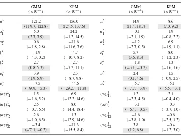
Table 2. Parameter estimates and corresponding confidence intervals for the GMM-based ANOVA model and the KPM-based ANOVA model. Here,μλandμδare the grand means of the birth rate and the death rate, respectively;αλi andαδi,ξjλandξjδ,ρkλandρkδare main effects of water, nitrogen, and blocks for the birth and death rates, respectively;(αξ )λijand(αξ )δijare interaction effects between water and nitrogen treatments for the birth and death rates, respectively, wherei, j, k=1,2.Confidence intervals are shaded in gray if they exclude zero.
GMM KPM GMM KPM
(×10−2) (×10−2) (×10−4) (×10−2)
μλ 121.2 156.0 μδ 14.9 8.6
(119.7, 122.8) (124.5, 137.6) (11.4, 18.7) (7.0, 9.2)
αλ1 5.0 24.2 α1δ −0.1 1.9
(2.7, 7.9) (−1.2, 14.5) (−2.1, 1.9) (−0.8, 2.2)
αλ2 0.6 −11.6 α2δ −1.2 6.9
(−1.8, 2.8) (−11.6, 7.6) (−2.7, 0.5) (−1.9, 1.1)
ξ1λ −1.9 −4.7 ξ1δ 5.7 8.0
(−4.3, 0.2) (−10.7, 8.2) (3.6, 8.3) (−1.2, 2.3)
ξ2λ 2.7 −2.7 ξ2δ −1.8 1.3
(0.8,5.3) (−7.2, 11.1) (−3.1,−0.2) (−1.6, 1.6)
ρ1λ 3.9 −2.3 ρ1δ 2.4 1.5
(1.9,6.9) (−8.7, 9.8) (0.1,4.6) (−0.9, 2.5)
ρ2λ −7.5 −44.6 ρ2δ −5.7 −5.1
(−9.9,−5.3) (−29.2,−11.8) (−7.7,−3.9) (−5.5,−3.1)
(αξ )λ11 1.5 6.9 (αξ )δ11 1.2 2.1
(−1.6, 5.2) (−12.2, 14.6) (−2.3, 4.5) (−0.4, 4.0)
(αξ )λ21 2.5 8.0 (αξ )δ21 −3.1 −0.3
(−0.7, 6.5) (−14.4, 18.4) (−6.4,−0.5) (−3.7, 1.0)
(αξ )λ12 2.6 1.3 (αξ )δ12 −1.6 −0.6
(−1.0, 6.5) (−12.9, 14.6) (−3.8, 1.0) (−2.5, 1.2)
(αξ )λ22 −3.4 −11.3 (αξ )δ22 3.8 −0.4
(−7.1,−0.2) (−15.5, 8.4) (1.2, 6.8) (−1.2, 3.0)
KPM-based model. This is mainly due to a larger power parametersˆ=2.3 for the GMM-based ANOVA model. The parameters can be interpreted as the usual ANOVA. For ex-ample, according to the fitted GMM-based ANOVA model, at low irrigation level, when the nitrogen treatment changes from the zero level to the variable level, the aphid birth rate increases from(121.2−1.9)×10−2=1.193 to (121.2+2.7)×10−2=1.239 (by around 3.9 %) and the death rate decreases from(14.9+5.7)×10−4=2.06×10⁻³to (14.9−1.8)×10−4=1.31×10⁻³(by around 36.4 %), therefore, the growth rate of aphid population is increased.
at the low irrigation level; the death rate of aphid population appears to be significantly higher under the no-nitrogen fertilization treatment; for both the birth and death rates, there are significant interaction effects between the medium irrigation level and the nitrogen levels. Although the KPM-based ANOVA model does not fit the data, confidence intervals for its parameters are also listed in Table2for completeness.
7. CONCLUSION
This paper develops a penalized spline method for estimating parameters of an ANOVA model of IDEs. The method does not require that the IDEs have analytic solutions, and also avoids using IDE numeric solvers. When the IDEs do not have analytic solutions, the clas-sical nonlinear regression method cannot be directly applied. The two-step method known in the literature first uses smoothing techniques to estimate the trajectories of the dynamic processes in the system and then applies the nonlinear regression. An important difference of the proposed penalized spline method is that it uses the IDEs as a regularization penalty when estimating the trajectories, and thus the estimated trajectories are implicit functions of the parameters. We developed a Gauss–Newton algorithm to minimize the nonlinear least squares criterion involving implicit functions. The results of our simulation studies indicate that the proposed method outperforms the two-step method in cases that the IDEs do not have analytic solutions, and performed comparably to the classical nonlinear re-gression in the special case that the IDEs have analytic solutions. In an application of the proposed method to an observed data set, we compared two mechanistic models in the literature, and our results suggest that the generalized mechanistic mode is better than the KPM in describing the dynamics of cotton aphids. ANOVA also enables us to gain insight into detection of treatment effects on the population dynamics of the cotton aphids.
APPENDIX A: NUMERICAL INTEGRATION METHODS
The integral term in (11) is essentially a double integral sinceFij k(t )= t
0h(Xij k(s)) ds. Both the inner and outer integrals usually do not have a closed-form expression, thus, they have to be calculated using numerical integration methods. In our implementation of the method, the outer integral is evaluated using the composite Simpson rule. The composite Simpson rule states that, for any given integrandf (t ),
tQ
t0
f (t ) dt≈δ
3
f (t0)+4 Q/2
q=1
f (t2q−1)+2 Q/2−1
q=1
f (t2q)+f (tQ)
,
t
0h(Xij k(s)) ds. For any given integrand,g(s), the composite trapezoidal rule is sP reduce the computational cost of extra function evaluation, we use the same set of quadra-ture points for calculating the inner and outer integrals. We use two different numerical integration methods for handling two integrals in order to reach a good balance between computational cost and accuracy. If Simpson’s rule is used for both the inner and outer integrals, we need more quadrature points in the inner integral and have to increase the computing load by evaluating the basis functions at these extra quadrature points; if the trapezoidal rule is used for both the inner and outer integrals, we will lose some numerical accuracy in the outer integral with the same number of quadrature points, because Simp-son’s rule is more accurate than the trapezoidal rule for numerical integration with the same number of quadrature points.
APPENDIX B: THE GAUSS–NEWTON ALGORITHM FOR
MINIMIZING
H (β)
Start with an initial guessβ(0)for the ANOVA parameterβ. The Gauss–Newton algo-rithm proceeds by the iterations
β(j+1)=β(j )−
Since the functioncij k(β)is usually an implicit function, it is hard to calculate the derivativedcij k/dβ. Fortunately, we can obtain an analytic expression for this derivative using the implicit function theorem as follows. Notice that the estimatecij k satisfies the identity
ACKNOWLEDGEMENTS
The authors would like to thank Prof. Montserrat Fuentes, the associate editor, and two reviewers for their very constructive suggestions and comments, which were extremely helpful for improving this paper.
[Received October 2011. Accepted March 2013. Published Online April 2013.]
REFERENCES
Barlow, N. D., and Dixon, A. F. G. (1980),Simulation of Lime Aphid Population Dynamics, Wageningen: Center for Agricultural Publishing and Documentation.
Blackman, R. L., and Eastop, V. F. (2000),Aphids on the World’s Crops: An Identification and Information Guide (2nd ed.), Chichester: Wiley.
Brunel, N. J.-B. (2008), “Parameter Estimation of ODE’s via Nonparametric Estimators,”Electronic Journal of Statistics, 2, 1242–1267.
Cao, J., Fussmann, G., and Ramsay, J. O. (2008), “Estimating a Predator–Prey Dynamical Model with the Param-eter Cascades Method,”Biometrics, 64, 959–967.
Cao, J., Huang, J. Z., and Wu, H. (2012), “Penalized Nonlinear Least Squares Estimation of Time-Varying Pa-rameters in Ordinary Differential Equations,”Journal of Computational and Graphical Statistics, 21, 42–56.
Chen, J., and Wu, H. (2008), “Efficient Local Estimation for Time-Varying Coefficients in Deterministic Dynamic Models with Applications to HIV-1 Dynamics,”Journal of the American Statistical Association, 103 (481), 369–383.
de Boor, C. (2001),A Practical Guide to Splines, New York: Springer.
Dixon, A. F. G. (1998),Aphid Ecology: An Optimization Approach(2nd ed.), London: Chapman and Hall.
Jones, B., and Nachtsheim, C. J. (2009), “Split-Plot Designs: What, Why, and How,”Journal of Quality Technol-ogy, 41, 340–361.
Kindlmann, P. (1985), “A Model of Aphid Population with Age Structure,” inMathematics in Biology and Medicine, Proceedings, Bari, 1983, eds. V. Capasso, E. Grosso and S. L. Paveri-Fontana, Berlin: Springer, pp. 72–77.
Kindlmann, P., Arditi, R., and Dixon, A. F. G. (2004), “A Simple Aphid Population Model,” inAphids in a New Millennium, eds. J. C. Simon, C. A. Dedryver, C. Rispe and M. Hulle, Paris: INRA, pp. 325–330.
Leclant, F., and Deguine, J. P. (1994), “Cotton Aphids,” inInsect Pests of Cotton, eds. G. A. Matthews and J. P. Tunstall, Wallingford: CAB International, pp. 285–323.
Mashanova, A., Gange, A. C., and Jansen, V. A. A. (2008), “Density-Dependent Dispersal May Explain the Mid-Season Crash in Some Aphid Populations,”Population Ecology, 50, 285–292.
Matis, J. H., Kiffe, T. R., Matis, T. I., and Stevenson, D. E. (2006), “Application of Population Growth Models Based on Cumulative Size to Pecan Aphids,”Journal of the Agricultural, Biological, and Environmental Statistics, 11, 425–449.
Matis, J. H., Kiffe, T. R., Matis, T. I., Jackman, J. A., and Singh, H. (2007a), “Population Size Models Based on Cumulative Size, with Application to Aphids,”Ecological Modelling, 205, 81–92.
Matis, J. H., Kiffe, T. R., Matis, T. I., and Stevenson, D. E. (2007b), “Stochastic Modeling of Aphid Population Growth with Nonlinear Powerlaw Dynamics,”Mathematical Biosciences, 208, 469–494.
Matis, J. H., Zhou, L., Kiffe, T. R., and Matis, T. I. (2007c), “Fitting Cumulative Size Mechanistic Models to Insect Population Data: A Nonlinear Mixed Effects Model Analysis,”Journal of the Indian Society of Agricultural Statistics, 61, 147–155.
Matis, T. I., Parajulee, M. N., Matis, J. H., and Shrestha, R. B. (2008), “A Mechanistic Model Based Analysis of Cotton Aphid Population Data,”Agricultural and Forest Entomology, 10, 355–362.
Prajneshu, C. S. (1998), “A Nonlinear Statistical Model for Aphid Population Growth,”Journal of the Indian Society of Agricultural Statistics, 51, 73–80.
Rabbinge, R., Ankersmit, G. W., and Pak, G. A. (1979), “Epidemiology and Simulation of Population Develop-ment of Sitobion Avenae in Winter Wheat,”Netherlands Journal of Plant Pathology, 85, 197–220.
Ramsay, J. O., and Silverman, B. W. (2005),Functional Data Analysis(2nd ed.), New York: Springer.
Ramsay, J. O., Hooker, G., Campbell, D., and Cao, J. (2007), “Parameter Estimation for Differential Equations: A Generalized Smoothing Approach (with discussion),”Journal of the Royal Statistical Society. Series B. Methodological, 69, 741–796.
Tatchell, G. M. (1989), “An Estimate of the Potential Economic Losses to Some Crops Due to Aphids in Britain,” Crop Protection, 8, 25–29.
Way, M. J. (1967), “The Nature and Causes of Annual Fluctuations in Numbers of Aphis Fabae Scop. on Field Beans (vicia Faba),”Annals of Applied Biology, 59, 175–188.