Statistical analysis of the covariance m

(1)

Statistical analysis of the covariance matrix MLE in

K-distributed clutter

Fre´de´ric Pascal

a,

, Alexandre Renaux

b a_{SONDRA/Supelec, 3 rue Joliot-Curie, F-91192 Gif-sur-Yvette Cedex, France}

b_{Laboratoire des Signaux et Systemes (L2S), Universite´ Paris-Sud XI (UPS), CNRS, SUPELEC, Gif-Sur-Yvette, France}

a r t i c l e

i n f o

Article history:

Received 22 January 2009 Received in revised form 13 July 2009

Accepted 26 September 2009 Available online 17 October 2009

Keywords:

Covariance matrix estimation Crame´r–Rao bound Maximum likelihood K-distribution

Spherically invariant random vector

a b s t r a c t

In the context of radar detection, the clutter covariance matrix estimation is an important point to design optimal detectors. While the Gaussian clutter case has been extensively studied, the new advances in radar technology show that non-Gaussian clutter models have to be considered. Among these models, thespherically invariant random vectormodelling is particularly interesting since it includes the K-distributed clutter model, known to fit very well with experimental data. This is why recent results in the literature focus on this distribution. More precisely, the maximum likelihood estimator of a K-distributed clutter covariance matrix has already been derived. This paper proposes a complete statistical performance analysis of this estimator through its consistency and its unbiasedness at finite number of samples. Moreover, the closed-form expression of the true Crame´r–Rao bound is derived for the K-distribution covariance matrix and the efficiency of the maximum likelihood estimator is emphasized by simulations.

Notations

The notational convention adopted is as follows: italic

indicates a scalar quantity, as in A; lower case boldface

indicates a vector quantity, as in a; upper case boldface

indicates a matrix quantity, as in A. RefAg and ImfAg

are the real and the imaginary parts of A, respectively.

The complex conjugation, the matrix transpose operator,

and the conjugate transpose operator are indicated by_,T_,

and H_{, respectively. The} _j _{th element of a vector} _a _is

denotedaðjÞ_{. The}_n_{th row and}_m_{th column element of the}

matrix A will be denoted by An;m. jAj and TrðAÞ are the

determinant and the trace of the matrixA, respectively.

denotes the Kronecker product._JJdenotes any matrix

norm. The operator vec(A) stacks the columns of the

matrixAone under another into a single column vector.

The operator vech(A), whereAis a symmetric matrix, does

the same things as vec(A) with the upper triangular

portion excluded. The operator veckðAÞ of a

skew-symmetric matrix (i.e.,AT

¼ A) does the same thing as

vechðAÞby omitting the diagonal elements. The identity

matrix, with appropriate dimensions, is denotedIand the

zero matrix is denoted 0. E½ denotes the expectation

operator.

-a:s:

stands for the almost sure convergence and

-Pr

stands for the convergence in probability. A zero-mean complex circular Gaussian distribution with covariance

matrixAis denotedCNð0;AÞ. A gamma distribution with

shape parameter k and scale parameter

y

is denoted

Gðk;

y

Þ. A complex m-variate K-distribution with

para-metersk,

y

, and covariance matrixAis denotedKmðk;

y

;AÞ.

A central chi-square distribution with kdegrees of

free-dom is denoted

w

2_ð_k_Þ_{. A uniform distribution with}

boundariesaandbis denotedU½a;b.

1. Introduction

The Gaussian assumption makes sense in many applications, e.g., sources localization in passive sonar, Contents lists available atScienceDirect

journal homepage:www.elsevier.com/locate/sigpro

Signal Processing

(2)

radar detection where thermal noise and clutter are generally modelled as Gaussian processes. In these contexts, Gaussian models have been thoroughly investi-gated in the framework of statistical estimation and detection theory (see, e.g., [1–3]). They have led to attractive algorithms such as the stochastic maximum likelihood method [4,5] or Bayesian estimators.

However, the assumption of Gaussian noise is not always valid. For instance, due to the recent evolution of radar technology, one can cite the area of space time adaptive processing-high resolution (STAP-HR) where the resolution is such that the central limit theorem cannot be applied anymore since the number of backscatters is too small. Equivalently, it is known that reﬂected signals can be very impulsive when they are collected by a low grazing angle radar [6,7]. This is why, in the last decades, the radar community has been very interested in problems dealing with non-Gaussian clutter modelling (see, e.g., [8–11]).

One of the most general non-Gaussian noise model is provided by spherically invariant random vectors (SIRV) which are a compound processes [12–14]. More precisely, an SIRV is the product of a Gaussian random vector (the so-called speckle) with the square root of a non-negative random scalar variable (the so-called texture). In other words, a noise modelled as an SIRV is a non-homogeneous Gaussian process with random power. Thus, these kind of processes are fully characterized by the texture and the unknown covariance matrix of the speckle. One of the major challenging difﬁculties in SIRV modelling is to

estimate these two unknown quantities [15]. These

problems have been investigated in [16]for the texture

estimation while [17,18] have proposed different estima-tion procedures for the covariance matrix. Moreover, the knowledge of these estimates accuracy is essential in radar detection since the covariance matrix and the texture are required to design the different detection schemes.

In this context, this paper focuses on parameters estimation performance where the clutter is modelled by a K-distribution. A K-distribution is an SIRV, with a gamma distributed texture depending on two real positive

parameters

a

and

b

. Consequently, a K-distribution

depends on

a

,

b

and on the covariance matrix M. This

model choice is justiﬁed by the fact that a lot of operational data experimentations have shown the good agreement between real data and the K-distribution model (see [7,19–22] and references herein).

This K-distribution model has been extensively studied in the literature. First, concerning the parameters estima-tion problem, [23,24] have estimated the gamma

dis-tribution parameters assuming that M is equal to the

identity matrix, [17]has proposed a recursive algorithm

for the covariance matrixMestimation assuming

a

and

b

known and [25] has used a parameter-expanded

expectation-maximization (PX-EM) algorithm for the

covariance matrix M estimation and for a parameter

n

assuming

n

¼

a

¼1=

b

. Note also that estimation schemes

in K-distribution context can be found in [26,27] and references herein. Second, concerning the statistical performance of these estimators, it has been proved in

[28]that the recursive scheme proposed by[17]converges

and has a unique solution which is the maximum likelihood (ML) estimator. Consequently, this estimator has become very attractive. In order to evaluate the

ultimate performance in terms of mean square error,[23]

has derived the true Crame´r–Rao Bound (CRB) for the

parameters of the gamma texture (namely,

a

and

b

)

assumingMequal to the identity matrix. Gini [29]has

derived the modiﬁed CRB on the one-lag correlation

coefﬁcient of M where the parameters of the gamma

texture are assumed to be nuisance parameters.

Concern-ing the covariance matrixM, a ﬁrst approach for the true

CRB study, which is known to be tighter than the modiﬁed

one, has been proposed in [25] whatever the texture

distribution. However, note that, for the particular case of

a gamma distributed texture, the analysis of[25]involves

several numerical integrations and no useful information concerning the structure of the Fisher information matrix (FIM) is given. Finally, classical covariance matrix

estima-tors are compared in[30]in the more general context of

SIRV.

The knowledge of an accurate covariance matrix estimate is of the utmost interest in context of radar detection since this matrix is always involved in the

detector expression [30]. Therefore, the goal of this

contribution is twofold. First, the covariance matrix ML estimate statistical analysis is provided in terms of consistency and bias. Second, the closed-form expression

of the true CRB for the covariance matrixMis given and is

analyzed. Finally, through a discussion and simulation results, classical estimation procedures in Gaussian and SIRV contexts are compared.

The paper is organized as follows. Section 2 presents the problem formulation while Sections 3 and 4 contain the main results of this paper: the ML estimate statistical performance in terms of consistency and bias and the derivation of the true CRB. Finally, Section 5 gives simulations which validate theoretical results.

2. Problem formulation

In radar detection, the basic problem consists in detecting if a known signal corrupted by an additive clutter is present or not. In order to estimate the clutter parameters before detection, it is generally assumed that

K signal-free independent measurements, traditionally

called the secondary datack,k¼1;. . .;Kare available.

As stated in the introduction, one considers a clutter modelled thanks to a K-distribution denoted

ckKmð

a

;ð2=

bÞ

2;MÞ: ð1Þ

From the SIRV deﬁnition,ckcan be written as

ck¼ ffiffiffiffiffi

t

k

p _xk

; ð2Þ

where

t

k is gamma distributed with parameters

a

and

ð2=

b

Þ2, i.e.,

t

kGð

a

;ð2=

b

Þ2Þ and, where xk is a complex

circular zero-mean m-dimensional Gaussian vector with

covariance matrix E½xkxH

k ¼M independent of

t

k. For

identiﬁability considerations,Mis normalized according

to TrðMÞ ¼m (see [17]). Note that the parameter

a

(3)

high the clutter tends to be Gaussian and, when

a

is small, the tail of the clutter becomes heavy.

The probability density function (PDF) of a random variable

t

kdistributed according toGð

a

;ð2=

b

Þ2Þis given by

pð

t

kÞ ¼

b

2 4

!a

t

a1

k

G

ð

a

Þexp

b

2 4

t

k

!

; ð3Þ

where

Gð

a

Þis the gamma function deﬁned by

G

ð

a

Þ ¼ Zþ1

0

xa1_exp_ð_x_Þ_dx_: _ð₄_Þ

From Eq. (2), the PDF ofckcan be written

pðck;M;

a

;

b

Þ ¼ Z þ1

0

1

t

m k

p

mjMj

exp c

H kM

1_ck

t

k !

pð

t

kÞd

t

k;

ð5Þ which is equal to

pðck;M;

a

;

b

Þ ¼

b

aþm

ðcH kM

1_ck

ÞðamÞ=2 2aþm1

p

m_j_M_j

G

_ð

a

_Þ Kma

b

ffiffiffiffiffiffiffiffiffiffiffiffiffiffiffiffiffiffiffi cH

kM

1_ck

q

;

ð6Þ

whereKnðÞis the modiﬁed Bessel function of the second

kind of order

n

[31].

Gini et al. have derived the ML estimator as the

solution of the following equation[17]:

^

MML¼1

K XK

k¼1

cmðcH kM^

1

MLckÞckc H

k; ð7Þ

where the functioncmðqÞis deﬁned as

cmðqÞ ¼₂p

b

ffiffiffi_q

Kam1ð

b

pffiffiffiqÞ

Kamð

b

pffiffiffiqÞ : ð

8Þ

Note that the ML estimate_MML^ _{has to be normalized as}

M:TrðMML^ Þ ¼m. Finally, it has been shown in[28]that

the solution to Eq. (7) exists and is unique for the aforementioned normalization.

3. Statistical analysis of_M^

ML

This section is devoted to the statistical analysis of_MML^

in terms of consistency and bias.

3.1. Consistency

An estimator_M^ _of_M_{is said to be consistent if}

JM^ MJ -Pr

K-þ10;

where K is the number of secondary data ck’s used to

estimateM.

Theorem 3.1 (_MML^ _consistency_). _MML^ _{is a consistent} estimate ofM.

Proof. In the sequel,_MML^ _{will be denoted}_M^_ð_K_Þ_{to show}

explicitly the dependence between_MML^ _{and the number}_K

ofxk0 _{s. Let us deﬁne the function}_fK;_M_{such that}

fK;M:

D!D;

A!1

K XK

k¼1

cmðcH kA

1_ck

ÞckcH k; 8

> > <

> > :

ð9Þ

where cmðÞ is deﬁned by Eq. (8), where D¼ fA2

Mmð

C

_Þj_AH_¼_A_;_A _{positive deﬁnite matrix} with} _Mm_ð

C

_{Þ ¼}

fmmmatrices with elements in

C

_g, and where

C

is the

set of complex scalar. As_M^_ð_K_Þ_{is a ﬁxed point of function}

fK;M, it is the unique zero, which respects the constraint TrðM^ðKÞÞ ¼m, of the following function:

gK: D!D;

A!gKðAÞ ¼AfK;MðAÞ: (

To prove the consistency of _M^_ð_K_Þ_{, Theorem 5.9 of}

[32, p. 46] will be used. First, the strong law of large numbers (SLLN) gives

8A2D; gKðAÞ -a:s:

K-þ1gðAÞ;

where

8A2D; gðAÞ ¼AE½cmðcH_A1_c

ÞccH

ð10Þ

forcKmð

a

;ð2=

b

Þ2;MÞ.

Let us now apply the change of variabley¼A1=2_c_{. We}

obtain

yKmð

a

;ð2=

b

Þ2;A1=2MA1=2Þ and

8A2D; gðAÞ ¼A1=2

ðIE½cmðyH_y

ÞyyH

ÞA1=2

and

8A2D; gKðAÞ ¼A1=2 _I

_K1X

K

k¼1

cmðyH kykÞykyHk

! A1=2_:

Let us verify the hypothesis of Theorem 5.9 of [32, p. 46]. We have to prove that for every

e

40,

ðH1Þ:sup

A2DfJ

gKðAÞ gðAÞJg -Pr

K-þ1 0;

ðH2Þ:_A inf

:JAMJZefJ

gðAÞJg40_¼g_ðM_Þ:

For everyA2D, we have

JgKðAÞ gðAÞJ¼JAJ 1 K

X K

k¼1

ðcmðyH

kykÞykyHk

E

½cmðyHyÞyyHÞ

:

Since E½cmðyH_y_Þ_yyH_o_{þ 1}_{, one can apply the SLLN to}

theKi.i.d. variablescmðyH

kykÞykyHk, with same ﬁrst order

moment. This ensuresðH1Þ.

Moreover, the functioncmðcH_A1_c

Þis strictly decreasing

w.r.t.A. Consequently,E½cmðcH_A1_c

ÞccH

too. This implies

thatE½cmðcH_A1_c

ÞccH_a_A_{, except for}_A_¼_M_{. This ensures}

ðH2Þ.

Finally, Theorem 5.9 of[32, p. 46]concludes the proof

and_MML^

-Pr

K-þ1 M. &

3.2. Bias

This subsection provides an analysis of the bias B

deﬁned byBðMML^ Þ ¼E½MML^ M.

(4)

Proof. For the sake of simplicity,_MML^ _{will be denoted}_M^ in this part. By applying the following change of variable, yk¼M1=2_ck_{, to Eq. (7), one has}

^ M¼_K1X

K

k¼1

cmðyH kT^

1

ykÞM1=2ykyHkM1=2;

where

^

T¼M1=2_MM^ 1=2

:

Therefore,

^ T¼1_KX

K

k¼1

cmðyH kT^

1

ykÞykyHk:

^

Tis thus the unique estimate (see[28, Theorem III.1]) of

the identity matrix, with TrðT^Þ ¼m. Its statistic is clearly

independent of M since the yk’s are i.i.d. SIRVs with a

gamma distributed texture and identity matrix for the

Gaussian covariance matrix. In other words,

ykKmð

a

;ð2=

bÞ

2;IÞ.

Moreover, for any unitary matrixU,

U_TU^ H

¼_K1X

K

k¼1

cmðzH kðUTU^

H

Þ1zkÞzkzH k;

where zk¼Uyk are also i.i.d. and distributed as

Kmð

a

;ð2=

b

Þ2;IÞandUTU^ H has the same distribution asT^. Consequently,

E½T^ ¼UE½T^UH _{for any unitary matrix}_U :

SinceE½T^is different from0, Lemma A.1 of[30]ensures

that E½T^ ¼

g

I for

g

2

R

. Remind that _T^_¼_M1=2_MM^ 1=2_,

thenE½M^ ¼

g

M. Moreover, since TrðM^Þ ¼TrðMÞ ¼m, one has

m¼EðTrðM^ÞÞ ¼TrðEðM^ÞÞ ¼

g

TrðMÞ ¼

g

m; ð11Þ

which implies that

g

¼1.

In conclusion,_M^ _{is an unbiased estimate of}_M_{, for any}

numberKof secondary data. &

3.3. Comments

Theorems 3.1 and 3.2 show the attractiveness of the estimator (7) in terms of statistical properties, i.e., consistency and unbiasedness. Note also that this estima-tor is robust since the unbiasedness property is at ﬁnite number of samples. In the next section, the Crame´r–Rao bound is derived for the observation model (2).

4. Crame´r–Rao bound

In this Section, the Crame´r–Rao bound w.r.t. M is

derived. The CRB gives the best variance that an unbiased estimator can achieve. The proposed bound will be compared to the mean square error of the previously studied ML estimator (Eq. (7)) in the next section.

The CRB for a parameter vector

h

is given by

CRBh¼ E

@2lnpðc1;. . .;cK;

h

Þ

@

h

@

h

T

1

; ð12Þ

where pðc1;. . .;cK;

h

Þ is the likelihood function of the

observationsck,k¼1;. . .;K. Concerning our model, the

parameter vector is

h

_{¼ ð}vechT

ðRefMgÞveckT

ðImfMgÞÞT; m21: ð13_Þ With the parametrization of Eq. (13), the structure of CRB becomes

CRBh¼

F1;1 F1;2

F2;1 F2;2

!1

; ð14_Þ

where theFi;j’s are the elements of the FIM given by

F1;1¼ E @ 2_ln_p_ð_c

1;. . .;cK;

h

Þ

@vechðRefMgÞ@vechTðRefMgÞ

" #

;

mðmþ1Þ

2

mðmþ1Þ

2 ; ð15Þ

F1;2¼FT2;1¼ E

@2_ln_p_ð_c

1;. . .;cK;

h

Þ

@vechðRefMgÞ@veckTðImfMgÞ

" #

;

mðmþ1Þ

2

mðm1Þ

2 ; ð16Þ

F2;2¼ E @ 2_ln_p_ð_c

1;. . .;cK;

h

Þ

@veckðImfMgÞ@veckTðImfMgÞ

" #

;

mðm1Þ

2

mðm1Þ

2 : ð17Þ

Since theck’s are i.i.d. random vectors, one have from

Eq. (6),

pðc1;. . .;cK;hÞ ¼ YK

k¼1

baþm ðcH

kM

1_c

kÞðamÞ=2 2aþm1

p

m_j_M_j_G_ð

a

_Þ Kmaðb

kM

1_c

k q

Þ:

ð18Þ Consequently, the log-likelihood function can be written as

lnpðc1;. . .;cKjhÞ ¼Kln b

aþm

2aþm1_pm_G_ð_a_Þ !

KlnðjM_jÞ

þXK k¼1

lnððcH

kM1ckÞðamÞ=2Kmaðb

kM 1_c

k q

ÞÞ:

ð19Þ

4.1. Result

The next subsections will show that the CRB w.r.t.

h

, in

this context, is given by

CRBh¼ 1 K

ðHT_FH

Þ1 ₀

0 ðKT_FK

Þ1

!

; ð20Þ

where the matricesHandKare constant transformation

matrices ﬁlled with ones and zeros such that vec_ðAÞ ¼

HvechðAÞ and vecðAÞ ¼KveckðAÞ, with A a

skew-sym-metric matrix, and where

F¼ ðMT

MÞ1 2ð

a

þ1Þ

mþ1

j

ð

a

;mÞ 8

ðMT

MÞ1=2_ð_I_þ_vec_ð_I_Þ_vecT

ðIÞÞðMT

MÞ1=2_; _ð₂₁_Þ

where

j

ð

a

;mÞis given by Eq. (F.3).

Remarks.

j

ð

a

;mÞis a constant which does not depend on

b

since

(5)

The ﬁrst term of the right hand side of Eq. (21) is the

Gaussian FIM (i.e., when

t

k¼1 8k). Indeed, using

Eqs. (24), (49) and (30),1 _{the Gaussian CRB, denoted}

GCRBh, is straightforwardly obtained as

GCRBh¼ 1 K

ðHT

ðMT

MÞ1_H

Þ1 ₀

0 ðKT

ðMT

MÞ1KÞ1 !

:

ð22_Þ By identiﬁcation with Eq. (21), it means that

lim

a-1

2ð

a

þ1Þ

mþ1

g

8

¼0:

Consequently, due to the structure ofIþvecðIÞvecT_ð_I_Þ_, the FIM for K-distributed observations is given by the

Gaussian FIM minus a sparse matrix depending on

a

,M

andm.

4.2. Outline of the proof

To make the reading easier, only the outline of the CRB derivation is given below. All the details are reported into the different appendices.

4.2.1. Analysis ofF1;1

With Eq. (19) one has

@2_ln_p_ð_c

1;. . .;cK;

h

Þ

@vech_ðRefMgÞ@vechT

ðRefMgÞ

¼ K @

2_ln_ðj_M_jÞ

þX

K

k¼1

@2_ln_ðð_cH kM

1_ck

ÞðamÞ=2Kmað

b

kM

1_ck

q

ÞÞ @vechðRefMgÞ@vechTðRefMgÞ : ð23Þ

The ﬁrst part of the right hand side of Eq. (23) is given by

K @

2_ln_ðj_M_jÞ

@vechðRefMgÞ@vechT_ðRefMgÞ ¼KHT

ðMT

MÞ1H ð24_Þ thanks to Appendix A, Eq. (A.3), and thanks to the fact that

@veckTðImfMgÞ

@vechðRefMgÞ ¼0 ð25Þ

and

@vechTðRefMgÞ

@vech_ðRefMgÞ ¼I: ð26Þ

Through the remain of the paper, let us set z¼

b

2cH kM

1_ck _and _f

ðzÞ ¼ln_ððz=

b

2ÞðamÞ=2KmaðpffiffiffizÞÞ. The

second term (inside the sum) of the right-hand side of

Eq. (23) is given by

@2_ln_ðð_cH kM

1_ck

ÞðamÞ=2Kmað

b

kM

1_ck

q

ÞÞ @vech_ðRefMgÞ@vechT_ðRefMgÞ

¼ @

2_f_ð_z_Þ

@vechðRefMgÞ@vechTðRefMgÞ: ð27Þ

Note that

@2fðzÞ ¼ @ @z

@fðzÞ @z @z

@z¼@

2_f_ð_z_Þ

@z2 @z@zþ

@fðzÞ @z @

2_z_; _ð₂₈_Þ

with (details are given in Appendix B)

@z¼ b2@vechTðRefMgÞHT

ðMT

MÞ1_vec_ð_ckcH kÞ

þi

b

2@veckTðImfMgÞKT

ðMT

MÞ1vecðckcH

kÞ ð29Þ and

@2z¼2

b

2@vechTðRefMgÞHT

ððMT_c

kc T kM

T

Þ

M1_Þ_H_@_vech_ð_R_e_f_M_gÞ

þ2

b

2@veckTðImfMgÞKT

ððMT_c

kcTkM T

Þ

M1

ÞK@veckðImfMgÞ ð30Þ and (details are given in Appendix C)

d1ðzÞ ¼@

fðzÞ

@z ¼

1 2 ffiffiffi

z

p Kmaþ1ð ffiffiffi z

p Þ

Kmaðpffiffiffiz Þ ð

31Þ

and

d2ðzÞ ¼@ 2_f_ð_z_Þ

@z2

¼₄1

z 1þ

Kmaþ1ðpffiffiffizÞ

Kmaðpffiffiffiz Þ

2 ffiffiffi z

p Kma1ð ffiffiffi z

p Þ

Kmaðpffiffiffiz Þ

: ð32Þ

Consequently, the structure of Eq. (28) becomes

@2fðzÞ ¼2

b

2d1ðzÞ@vechTðRefMgÞHTP1H@vechðRefMgÞ

þ2

b

2d1ðzÞ@veckTðImfMgÞKTP1K@veckðImfMgÞ

þ

b

4d2ðzÞ@vechTðRefMgÞHTP2H@vechðRefMgÞ

þ

b

4d2ðzÞ@veckTðImfMgÞKTP2K@veckðImfMgÞ;

ð33Þ

where

P1¼ ðMTckc T kM

T

Þ M1_; _ð₃₄_Þ

P2¼ ðMTMÞ1vecðckcHkÞvecHðckcHkÞðM T

MÞ1: ð35_Þ Therefore, Eq. (27) is given by

@2_f_ð_z_Þ

¼2

b

2d1ðzÞHTP1Hþ

b

4d2ðzÞHTP2H ð36Þ

due to Eqs. (25) and (26).

Using Eqs. (23), (24), and (36),F1;1is given by

F1;1¼ KHTððMTMÞ1þ2

b

2E½d1ðzÞP1

þ

b

4E½d2ðzÞP2ÞH; ð37Þ

whered1ðzÞand d2ðzÞare deﬁned by Eqs. (31) and (32),

respectively. 1_With_b2

¼1,z¼cH

kM

1_c

kwhich is the term to be derived w.r.t.hin

(6)

The two expectation operators involved in the previous equation can be detailed as follows:

E½d1ðzÞP1 ¼ 12ðM

T

CM

T

Þ M1

ð38Þ

and

E½d2ðzÞP2 ¼14ðM

T

MÞ1ð

W

þ

N

!

ÞðMT

MÞ1; ð39Þ where

C

¼E 1ffiffiffi z

p Þ

KmaðpffiffiffizÞ c

kc T k

;

W

¼E 1 zvecðckc

H

kÞvecHðckcHkÞ

;

N

¼E 2 z3=2

KmaðpffiffiffizÞ

vecðckcH

kÞvecHðckcHkÞ

;

!

¼E 1 z

Kma1ðpffiffiffizÞKmaþ1ðpffiffiffizÞ

K2

mað

ffiffiffi z

p

Þ vecðckc

H kÞvec

H

ðckcH kÞ:

8 > > > > > > > > > > > > > <

> > > > > > > > > > > > > :

ð40_Þ After some calculus detailed in Appendix D, one ﬁnds

C

¼ 2

b

2M

T

: ð41Þ

Concerning

W

, one has

W

¼ 1

b

2E

vec_ðckcH kÞvec

H

ðckcH kÞ cH

kM

1_ck

" #

; ð42Þ

where the expectation is taken under a complex K-distributionKmð

a

;ð2=

b

Þ2;MÞ.

Concerning

N

, one has

N

¼ 1 ð

a

1_Þ

b

2E

vecðckcH

kÞvecHðckcHkÞ cH

kM

1_ck

" #

; ð43_Þ

a

1;ð2=

b

Þ2;MÞ.

Concerning

!

, one has

!

¼ 1

b

2E

Kma1ðpffiffiffizÞKmaþ1ðpffiffiffizÞ

K2

mað

ffiffiffi z

p Þ

vecðckcH

kÞvecHðckcHkÞ cH

kM

1_ck

" #

;

ð44_Þ

a

;ð2=

b

Þ2;MÞ.

The closed-form expression of EvecðckcH

kÞvecHðckcHkÞ=

cH kM

1_ck

under a complex K-distribution is given in

Appendix E. One ﬁnds

W

¼ 8

b

4

a

mþ1ðM T=2

M1=2

ÞðIþvecðIÞvecT

ðIÞÞðMT=2

M1=2

Þ

ð45Þ

and

N

¼ 8

b

4

1 mþ1ðM

T=2

M1=2

ÞðI_þvecðI_ÞvecT

ðI_ÞÞðMT=2

M1=2

Þ:

ð46Þ

The structure of

!

is analyzed in Appendix F.

Consequently, Eq. (37) is reduced to

F1;1¼KHT ðMTMÞ1

2ð

a

þ1Þ

mþ1

j

ð

a

;mÞ 8

ðMT

MÞ1=2ðIþvecðIÞvecT

ðIÞÞðMT

MÞ1=2 H; ð47Þ

where

j

ð

a

;mÞis given by Eq. (F.3).

4.2.2. Analysis ofF2;2

The analysis ofF2;2is similar to the one used forF1;1.

Indeed, one has to calculate

@2_ln_p_ð_c

1;. . .;cK;

h

Þ

@veckðImfMgÞ@veckTðImfMgÞ

¼ K @

2_ln_ðj_M_jÞ

@veck_ðImfMgÞ@veckT_ðImfMgÞ

þX

K

k¼1

@2_ln_ðð_cH kM

1_ck

ÞðamÞ=2Kmað

b

kM

1_ck

q

ÞÞ @veck_ðImfMgÞ@veckT_ðImfMgÞ : ð48Þ Using Eq. (A.3), one has

K @2lnðjMjÞ

@veckðImfMgÞ@veckTðImfMgÞ ¼KKT

ðMT

MÞ1_K _ð₄₉_Þ

due to Eq. (25) and due to

@veckðImfMgÞ

@veckTðImfMgÞ¼I: ð50Þ

By using the same notation as for the derivation ofF1;1

and by using Eq. (33), one obtains for the second term on the right hand side of Eq. (48) as

@2lnððcH kM

1_ck

ÞðamÞ=2Kmað

b

kM

1_ck

q

ÞÞ @veckðImfMgÞ@veckTðImfMgÞ

¼2

b

2d1ðzÞKTP1Kþ

b

4d2ðzÞKTP2K; ð51Þ

whereP1,P2,d1ðzÞandd2ðzÞare deﬁned by Eqs. (34), (35),

(31), and (32), respectively. Therefore, the structure ofF2;2

is the same as the structure of F1;1 except that one

replaces the matrixHby the matrixK.

4.2.3. Analysis ofF1;2¼FT2;1

Due to the structure of Eq. (A.3) and Eq. (33), and since the derivation is w.r.t.@vechðRefMgÞand@veckTðImfMgÞ, it is clear that

F1;2¼FT2;1¼0 ð52Þ

by using Eq. (25).

This concludes the proof of the CRB derivation.

5. Simulation results

In this section, some simulations are provided in order to illustrate the proposed previous results in terms of consistency, bias, and variance analysis (throughout the CRB). While no mathematical proof is given in other sections, we show the efﬁciency of the MLE meaning that the CRB is achieved by the variance of the MLE.

The results presented are obtained for complex

K-distributed clutter with covariance matrixMrandomly

(7)

All the results are presented different values of

parameter

a

and

b

¼2pffiffiffi

a

following the scenario of[17].

The size of each vector ck ism¼3. Remember that the

parameter

a

represents the spikiness of the clutter (when

a

is high the clutter tends to be Gaussian and, when

a

is

small, the tail of the clutter becomes heavy). The norm

used for consistency and bias is theL2_norm.

5.1. Consistency

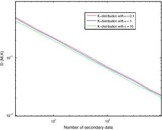
Fig. 1 presents results of MLE consistency for 1000

Monte Carlo runs per each value ofK. For that purpose, a

plot ofDðM^;KÞ ¼JM^ MJversus the numberKofck’s is

presented for each estimate. It can be noticed that the

[image:7.544.110.430.142.399.2]

above criterionDðM^;KÞtends to 0 whenKtends to1for

[image:7.544.112.432.433.677.2]

Fig. 1.Dð_M^_;_KÞ_{versus the number of secondary data for different values of}_a_.

(8)

each estimate. Moreover, note that the parameter

a

has very few inﬂuence on the convergence speed which highlights the robustness of the MLE.

5.2. Bias

Fig. 2shows the bias of each estimate for the different

values of

a

. The number of Monte Carlo runs is given in

the legend of the ﬁgure. For that purpose, a plot of the criterionCðM^;KÞ ¼JM^

___

MJversus the numberKofck’s is

presented for each estimate._M___^ _{is deﬁned as the empirical}

mean of the quantities_M^_ð_i_Þ_{obtained from}_I_{Monte Carlo}

runs. For each iterationi, a new set ofKsecondary datack

is generated to compute M^ðiÞ. It can be noticed that,

as enlightened by the previous theoretical analysis, the

bias of_M^ _{tends to 0 whatever the value of}_K_{. Furthermore,}

one sees again the weak inﬂuence of the parameter

a

on

the unbiasedness of the MLE.

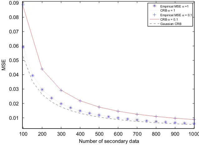
5.3. CRB and MSE

The CRB and empirical variance of the MLE for 10 000

Monte Carlo runs are plotted inFig. 3. For comparison, we

also plot the Gaussian CRB (i.e., when

t

k¼18k) given by

Eq. (22). Although it is not mathematically proved in this

paper, one observes, in Fig. 3, the efﬁciency of the MLE

even for impulsive noise (

a

small).

6. Conclusion

In this paper, a statistical analysis of the maximum likelihood estimator of the covariance matrix of a complex multivariate K-distributed process has been proposed. More particularly, the consistency and the unbiasedness

(at finite number of samples) have been proved. In order to analyze the variance of the estimator, the Crame´r–Rao lower bound is derived. The Fisher information matrix in this case is simply the Fisher information matrix of the Gaussian case plus a term depending on the tail of the K-distribution. Simulation results have been proposed to illustrate these theoretical analyses. These results have shown the efficiency of the estimator and the weak influence of the spikiness parameter in terms of consis-tency and bias.

Appendix A. Derivation of@2lnfjMjg

To ﬁnd this term and several other, we will use the

following results[33]:

@TrðXÞ ¼Trð@XÞ; ðA:1aÞ

@vecðXÞ ¼vecð@XÞ; ðA:1bÞ

@A1

¼ A1_@_AA1_;

ðA:1cÞ

@jAj ¼ jAjTrðA1

@AÞ; ðA:1dÞ

@ðA BÞ ¼@ðAÞ BþA @ðBÞ where ¼ or ðA:1eÞ

@lnðjMjÞ ¼TrðM1_@_M_Þ_; _ð_A_:_1f_Þ

@ð@MÞ ¼0; ðA:1gÞ

TrðABÞ ¼TrðBAÞ ðA:1hÞ

M1

¼ ðMMÞ1; ðA:1iÞ

Tr_ðAH_B

Þ ¼vecH

ðAÞvec_ðBÞ; ðA:1j_Þ

100 200 300 400 500 600 700 800 900 1000

0.01 0.02 0.03 0.04 0.05 0.06 0.07 0.08 0.09

Number of secondary data

MSE

[image:8.544.113.432.56.290.2]

Empirical MSE α =1 CRB α = 1 Empirical MSE α = 0.1 CRB α = 0.1 Gaussian CRB

(9)

vecðABCÞ ¼ ðCT

AÞvecðBÞ: ðA:1kÞ By using these properties, one has

@lnðjMjÞ ¼TrðM1

ð@MÞÞ fromðA:1fÞ

@2lnðjMjÞ ¼ TrðM1

ð@MÞM1

@MÞ fromðA:1aÞðA:1eÞðA:1gÞðA:1cÞ ¼ vecH

ðM1

ð@MÞM1

Þvecð@MÞ fromðA:1jÞ ¼ vecH

ð@MÞðMT

M1

ÞHvecð@MÞ fromðA:1kÞ

¼ @vecH

ðMÞðMT

MÞ1@vec_ðMÞ from_ðA:1b_ÞðA:1i_Þ:

By lettingM¼RefMg þiImfMgin Eq. (A.3), one has

@2lnðjMjÞ ¼ @vecH

ðRefMg þiImfMgÞ ðMT

MÞ1@vec_ðRefMg þiImfMgÞ ¼ @vecH

ðRefMgÞðMT

MÞ1@vecðRefMgÞ @vecH

ðiImfMgÞðMT

MÞ1@vecðRefMgÞ @vecH_ð_R_e_f_M_gÞð_MT

MÞ1_@_vec_ð_i_I_m_f_M_gÞ

@vecH

ðiImfMgÞðMT

MÞ1@vec_ðiImfMgÞ: ðA:2Þ Since vecH_ð_i_I_m_f_M_{gÞ ¼}_i_vecT_ð_I_m_f_M_gÞ_{and vec}H_ð_R_e_f_M_gÞ

¼vecT_ð_R_e_f_M_gÞ_,_@2_ln_ðj_M_jÞ_{is reduced to}

@2_ln_ðj_M_{jÞ ¼}_@_vecT

ðRefMgÞðMT

MÞ1@vecðRefMgÞ @vecT

ðImfMgÞðMT

MÞ1@vecðImfMgÞ ¼ @vechTðRefMgÞHT

ðMT

MÞ1H@vechðRefMgÞ @veckTðImfMgÞKT

ðMT

MÞ1K@veckðImfMgÞ; ðA:3Þ

where the matrix H and Kare constant transformation

matrices ﬁlled with ones and zeros such that vec_ðAÞ ¼

HvechðAÞand vecðAÞ ¼KveckðAÞ.

Appendix B. Derivation of@zand@2z

By using the properties from Eq. (A.1a) to (A.1k), one

has for@z

@z¼

b

2@ðcH kM

1_ck

Þ ¼

b

2@TrðcH kM

1_ck

Þ

¼

b

2Tr_ðcH

k@ðM1ÞckÞ fromðA:1aÞ

¼

b

2TrðcH kM

1

@MM1_ck

Þ fromðA:1cÞ

¼

b

2Trð@MM1_ckcH

kM1Þ fromðA:1hÞ

¼ b2vecH

ð@MÞvecðM1_ckcH

kM1Þ fromðA:1jÞ

¼

b

2@vecH

ðMÞ

ðMT

MÞ1vecðckcH

kÞ fromðA:1bÞðA:1kÞðA:1iÞ: By lettingM¼RefMg þiImfMg, one obtains

@z¼

b

2@vecT

ðRefMgÞðMT

MÞ1vecðckcH kÞ

þi

b

2@vecT

ðImfMgÞðMT

MÞ1_vec_ð_ckcH kÞ

¼

b

2@vechTðRefMgÞHT

ðMT

MÞ1vecðckcH kÞ

þi

b

2@veckT_ðImfMgÞKT

ðMT

MÞ1vec_ðckcH

kÞ: ðB:1Þ

Concerning@2z, one has

@z¼

b

2TrðcH

kM1@MM1ckÞ ðB:2Þ

@2_z_¼

b

2

TrðcH

k@ðM1@MM1ÞckÞ fromðA:1aÞ

¼

b

2TrðcH

k@ðM1Þ@MM1ck

þcH

kM1@M@ðM1ÞckÞ fromðA:1eÞðA:1gÞ

¼2

b

2Trð@MM1_@_MM1_ckcH

kM1Þ fromðA:1cÞðA:1hÞ

¼2

b

2@vecH

ðMÞððMT_c

kc T kM

T

Þ

M1_Þ_@_vec_ð_M_Þ _from_ð_A_:_1j_Þð_A_:_1k_Þð_A_:_1b_Þ

By lettingM¼RefMg þiImfMg, one obtains

@2z¼2b2@vechTðRefMgÞHT ððMT_c

kcTkMTÞM1ÞH@vechðRefMgÞ þ2

b

2@veckT_ðImfMgÞKT

ððMT_c

kcTkM T

Þ

M1_Þ_K_@_veck_ð_I_m_f_M_gÞ_: _ð_B_:₃_Þ

Appendix C. Derivation of@fðzÞ=@zand@2_f_ð_z_Þ_=@_z2

Concerning the ﬁrst derivative offðzÞ, one has

@fðzÞ

@z ¼

@ @zlnððz=

b

2

ÞðamÞ=2_Km

aðpffiffiffizÞÞ

¼

a

₂ m

z þ

1 KmaðpffiffiffizÞ

@KmaðpffiffiffizÞ

@z : ðC:1Þ

Since@KnðyÞ=@y¼ Knþ1ðyÞ þ ð

n

=yÞKnðyÞ[34]. It follows

that

@KmaðpffiffiffizÞ

@z ¼

1 2 ffiffiffi

z

p Kmaþ1ð

ffiffiffi z

p

Þ þm₂_z

a

KmaðpffiffiffizÞ: ðC:2Þ

Plugging Eq. (C.2) in Eq. (C.1), one obtains

@fðzÞ

@z ¼

1 2 ffiffiffi

z

p Þ

KmaðpffiffiffizÞ : ð

C:3Þ

Concerning the second derivative offðzÞ, one has

@2_f_ð_z_Þ

@z2 ¼

1 2 @ @z

1 ffiffiffi z

p Þ

Kmaðpffiffiffiz Þ

¼₄_z1₃=2

KmaðpffiffiffizÞ

1 4z

@ @y

Kmaþ1ðyÞ

KmaðyÞ

y¼pﬃﬃ_z !

: ðC:4Þ

Since@KnðyÞ=@y¼ Kn1ðyÞ ð

n

=yÞKnðyÞ[34]. It follows

that

@ @y

Kmaþ1ðyÞ KmaðyÞ

_y

¼pﬃﬃ_z

¼

ðKmaðpffiffiffizÞ þm

a

ffiffiffiþ1 z

p Kmaþ1ðpzffiffiffiÞÞKmaðpffiffiffizÞ K2

mað

ffiffiffi z

p Þ

þ

Kmaþ1ðpffiffiffizÞðKma1ðpffiffiffizÞ þ

m

a

ffiffiffi z

p KmaðpffiffiffizÞÞ

K2

mað ffiffiffiz

p

Þ : ðC:5Þ Plugging Eq. (C.5) in Eq. (C.4), one obtains

@2_f_ð_z_Þ

@z2 ¼

1 4zþ

1 2z3=2

KmaðpffiffiffizÞ

1 4z

Kmaþ1ðpffiffiffizÞKma1ðpffiffiffizÞ

K2

mað

ffiffiffi z

p

(10)

Appendix D. Derivation of matrix

C

The matrix

C

is given by

C

¼E 1ffiffiffi z

p Þ

KmaðpffiffiffizÞ c

kcTk

¼

Gð

₂

a

G

1Þ ð

a

Þ E

T

½ckcH

k; ðD:1Þ

where the last expectation is taken under the distribution

pðckÞ ¼

b

aþm1

jMj1

2aþm2

p

m

G

_ð

a

₁_Þðc H

kM1ckÞða m1Þ=2

Kmaþ1ð

b

kM

1_ck

q

Þ; ðD:2Þ

which is a complex K-distribution Kmð

a

1;ð2=

b

Þ2;MÞ.

Then

C

¼₂ 1 ð

a

1_ÞE

T

½ckcH k ¼

1 2_ð

a

1_ÞE

T

½

t

kxkxH k

¼₂ 1

ð

a

1_ÞE½

t

kET½xkxHk; ðD:3Þ

where E½

t

k ¼ ð

a

1Þð2=

bÞ

2 since

t

k follows a Gamma

distributionGð

a

1;ð2=

b

Þ2ÞandET_½_xkxH k ¼M

T_since_xk_is

a complex normal random vector (independent of

t

k) with

zero mean and covariance matrix M. Consequently,

C

¼ ð2=

b

2ÞMT_.

Appendix E. Derivation of

E½vecðckcHkÞvec H

ðckcHkÞ=c H kM

1_c

k

In this appendix, we derive the expression ofE½vecðckcH

kÞ vecH_ð_ckcH

kÞ=cHkM

1_ck

whereckKmð

a

;ð2=

b

Þ2;MÞ. The case whereckKmð

a

1;ð2=

b

Þ2;MÞwill be, of course, straight-forward. Let us set the following change of variable:

ck¼M1=2_yk_{. One obtains from Eq. (A.1k)}

E vecðckc

H

kÞvecHðckcHkÞ

cH

kM

1_c

k

" # ¼ ðMT=2

M1=2 Þ

E vecðyky H

kÞvecHðykyHkÞ yH

kyk

" #

ðMT=2

M1=2

Þ; ðE:1Þ

where ykKmð

a

;ð2=

bÞ

2;IÞ. Since yk¼pffiffiffiffiffi

t

kxk, where

t

kGð

a

;ð2=

b

Þ2Þis independent ofxkCNð0;IÞ, one has

E vecðckc H

kÞvecHðckcHkÞ cH

kM

1_ck

" #

¼ ðMT=2

M1=2

ÞE½

t

kR

ðMT=2

M1=2

Þ; ðE:2Þ whereE½

t

k ¼

a

ð2=

bÞ

2and where

R¼E vecðxkx H

kÞvecHðxkxHkÞ xH

kxk

" #

: ðE:3Þ

Let us setxðjÞ

k ¼ ffiffiffiffiffiffi

r

2

j q

expði

y

jÞforj¼1;. . .;m. Note that

r

2

j

w

2ð2Þ is independent of

y

jU½0;2p. Consequently, the

elements of the matrixRcan be rewritten as

Rk;l¼E

ffiffiffiffiffiffiffiffiffiffiffiffiffiffiffiffiffiffiffiffiffiffiffiffi

r

2

p

r

2q

r

2p0

r

2q0 q

Pm j¼1

r

2j 2

4

3

5E½expðið

y

p

y

p0þ

y

q0

y

qÞÞ ðE:4Þ

since

xH kxk¼

X m

j¼1

r

2

j and½vecðxkxHkÞn

¼ ffiffiffiffiffiffiffiffiffiffiffiffi

r

2

p

r

2p0 q

expðiðyp

y

p0ÞÞ: ðE:5Þ

Note thatE½expðið

y

p

y

p0þ

y

q0

y

qÞÞa0 if and only if

(1) p¼p0_¼_q_¼_q0_{, i.e.,}_l_¼_k_¼_p_þ_m_ð_p₁_Þ_,

(2) p¼p0_,_q_¼_q0_and_p_a_q_{, i.e.,}_l_¼_k_¼_p_þ_m_ð_q₁_Þ_,

(3) p¼q,p0_¼_q0_and_p_a_p0_{, i.e.,}_l_¼_p0_þ_m_ð_p0₁_Þ_and

k¼pþmðp1Þ.

Consequently, the non-zero elements ofRk;lare given by

(1) Rp_þmðp1Þ;pþmðp1Þ¼E½ð

r

2pÞ2= Pm

j¼1

r

2j ¼4=ðmþ1Þ, (2) Rpþmðq1Þ;pþmðq1Þ¼E½

r

2p

r

2p0=

Pm

j¼1

r

2j ¼2=ðmþ1Þ, (3) Rpþmðp1Þ;p0_þmðp01Þ¼E½

r

2p

r

2q=

Pm

j¼1

r

2j ¼2=ðmþ1Þ,

and the matrix E½vecðckcH

kÞvecHðckcHkÞ=cHkM1ck can be written as

E vecðckc H

kÞvecHðckcHkÞ cH

kM

1_ck

" #

¼_m2

a

þ1

2

b

2

ðMT=2

M1=2

Þ ðIþvecðIÞvecT

ðIÞÞðMT=2_M1=2_Þ_:

ðE:6Þ

In the same way, the expression of E½vecðckcH

kÞ vecH_ð_ckcH

kÞ=cHkM

1_ck

where ckKmð

a

1;ð2=

b

Þ2;MÞ is given by

E vecðckc H

kÞvecHðckcHkÞ cH

kM

1_ck

" #

¼2_mð

a

1Þ þ1

2

b

2

ðMT=2

M1=2

Þ ðIþvecðIÞvecT

ðIÞÞðMT=2

M1=2

Þ: ðE:7Þ

Appendix F. Analysis of

!

Let us set the following change of variable: ck¼

M1=2 ffiffiffiffiffi

t

k

p _xk_{, where}

t

kGð

a

;ð2=

b

Þ2Þ is independent of xkCNð0;IÞ, one has

!

¼ 1

b

2ðM

T=2

M1=2

Þ

!

~ðMT=2

M1=2

Þ;

where

~

!¼E tkKma1ðb ffiffiffiffiffiffiffiffiffiffiffiffiffiffiffi tkxHkxk

q

ÞKmaþ1ðb ffiffiffiffiffiffiffiffiffiffiffiffiffiffiffi tkxHkxk

q Þ

K2

maðb ffiffiffiffiffiffiffiffiffiffiffiffiffiffiffi tkxHkxk

q Þ

vecðxkxHkÞvecHðxkxHkÞ

xH kxk

2 6 4 3 7 5:

ðF:1Þ

Let us setxðjÞ

k ¼ ffiffiffiffiffiffi

r

2

j q

expði

y

jÞforj¼1;. . .;m.

r

2j

w

2ð2Þis

independent of

y

jU½0;2p. Consequently, due to Eq. (E.5),

the elements of the matrix

!

~ _{can be rewritten as}

~ Uk;l¼E tk0

Kma1 b

ffiffiffiffiffiffiffiffiffiffiffiffiffiffiffiffiffiffiffiffiffiffiffiffi tk0Pm_j_¼₁r2_j

q

Kmaþ1 b

q

K2

ma b

q

ffiffiffiffiffiffiffiffiffiffiffiffiffiffiffiffiffiffiffiffiffiffiffiffi r2

pr2qr2p0r2q0

q

Pm j¼1r2j

2 6 4 3 7 5

(11)

As before,E½expðið

y

p

y

p0þ

y

q0

y

qÞÞa0 if and only if

(1) p¼p0_¼_q_¼_q0_{, i.e.,}_l_¼_k_¼_p_þ_m_ð_p₁_Þ_,

(2) p¼p0_,_q_¼_q0_and_p_a_q_{, i.e.,}_l_¼_k_¼_p_þ_m_ð_q₁_Þ_,

(3) p¼q,p0_¼_q0_and_p_a_p0_{, i.e.,}_l_¼_p0_þ_m_ð_p0₁_Þ_and

k¼pþmðp1_Þ.

Consequently, the non-zero elements of

U

~

k;lare given by

(1)

U

~pþmðp1Þ;pþmðp1Þ

¼E tk0 Kma1 b

q

Kmaþ1 b

q

K2

ma b

q

ðr2

pÞ2

Pm j¼1r2j

2

6 4

3

7 5;

(2)

U

~pþmðq1Þ;pþmðq1Þ

¼E tk0 Kma1 b

q

Kmaþ1 b

q

K2

ma b

q

r2

pr2p0

Pm j¼1r2j

2

6 4

3

7 5;

(3)

U

~pþmðp1Þ;p0_þmðp01Þ

¼E tk0 Kma1 b

ffiffiffiffiffiffiffiffiffiffiffiffiffiffiffiffiffiffiffiffiffiffiffiffi tk0Pm_j_¼1r2j

q

Kmaþ1 b

ffiffiffiffiffiffiffiffiffiffiffiffiffiffiffiffiffiffiffiffiffiffiffiffi tk0Pm_j_¼1r2j

q

K2

ma b

q

r2

pr2q

Pm j¼1r2j

2

6 4

3

7 5:

Note that

U

~

pþmðq1Þ;pþmðq1Þ¼

U

~pþmðp1Þ;p0_þmðp01Þ¼

1

2

U

~pþmðp1Þ;pþmðp1Þ8p8p0 8q8q0. Consequently, only

j

ð

a

;mÞ

¼b2E tk0 Kma1 b

tk0

Pm

j¼1r2j q

Kmaþ1ðb

tk0

Pm

j¼1r2j q

Þ

K2

maðb

tk0Pmj¼1r2j q

Þ

ðr2

pÞ2

Pm

j¼1r2j 2

6 4

3

7 5

ðF:3Þ

has to be computed and the matrix

!

can be written as

!

¼

j

ð

a

;mÞ

2

b

4 ðM

T=2

M1=2

ÞðIþvec_ðIÞvecT

ðIÞÞ

ðMT=2

M1=2

Þ: ðF:4_Þ

Note that

j

ð

a

;mÞ is independent of

b

since,

b

2

t

k0Gð

a

;4Þ.

References

[1] S.M. Kay, Fundamentals of Statistical Signal Processing—Detection

Theory, vol. 2, Prentice-Hall, PTR, Englewood Cliffs, New Jersey, 1998.

[2] H.L. Van Trees, Detection Estimation and Modulation Theory, Part I, Wiley, New York, 1968.

[3] L.L. Scharf, D.W. Lytle, Signal detection in Gaussian noise of unknown level: an invariance application, IEEE Trans. Inf. Theory 17 (1971) 404–411.

[4] S. Haykin, Array Signal Processing, Prentice-Hall Signal Processing Series, Prentice-Hall, Englewood Cliffs, New Jersey, 1985. [5] H.L. Van Trees, Detection, Estimation and Modulation Theory, Part

IV: Optimum Array Processing, Wiley, New York, 2002.

[6] J.B. Billingsley, Ground clutter measurements for surface-sited radar, Technical Report 780, MIT, February 1993.

[7] A. Farina, F. Gini, M.V. Greco, L. Verrazzani, High resolution sea clutter data: a statistical analysis of recorded live data, IEE Proc. Part F 144 (3) (1997) 121–130.

[8] E. Conte, M. Longo, Characterization of radar clutter as a spherically invariant random process, IEE Proc. Part F 134 (2) (1987) 191–197.

[9] K.J. Sangston, K.R. Gerlach, Coherent detection of radar targets in a non-Gaussian background, IEEE Trans. Aerosp. Electron. Syst. 30 (1994) 330–340.

[10] F. Gini, Sub-optimum coherent radar detection in a mixture of K-distributed and Gaussian clutter, IEE Proc. Radar Sonar Navigation 144 (1) (1997) 39–48.

[11] F. Gini, M.V. Greco, M. Diani, L. Verrazzani, Performance analysis of two adaptive radar detectors against non-Gaussian real sea clutter data, IEEE Trans. Aerosp. Electron. Syst. 36 (4) (2000) 1429–1439. [12] B. Picinbono, Spherically invariant and compound Gaussian

stochastic processes, IEEE Trans. Inf. Theory (1970) 77–79. [13] K. Yao, A representation theorem and its applications to spherically

invariant random processes, IEEE Trans. Inf. Theory 19 (5) (1973) 600–608.

[14] M. Rangaswamy, D.D. Weiner, A. Ozturk, Non-Gaussian vector identiﬁcation using spherically invariant random processes, IEEE Trans. Aerosp. Electron. Syst. 29 (1) (1993) 111–124.

[15] M. Rangaswamy, Statistical analysis of the nonhomogeneity detector for non-Gaussian interference backgrounds, IEEE Trans. Signal Process. 53 (6) (2005) 2101–2111.

[16] E. Jay, J.-P. Ovarlez, D. Declercq, P. Duvaut, Bord: Bayesian optimum radar detector, Signal Process. 83 (6) (2003) 1151–1162.

[17] F. Gini, M.V. Greco, Covariance matrix estimation for CFAR detection in correlated heavy tailed clutter, Signal Process. 82 (12) (2002) 1847–1859 (special section on SP with Heavy Tailed Distributions). [18] E. Conte, A. DeMaio, G. Ricci, Recursive estimation of the covariance matrix of a compound-Gaussian process and its application to adaptive CFAR detection, IEEE Trans. Signal Process. 50 (8) (2002) 1908–1915.

[19] S. Watts, Radar detection prediction in sea clutter using the compound K-distribution model, IEE Proc. Part F 132 (7) (1985) 613–620.

[20] T. Nohara, S. Haykin, Canada east coast trials and the K-distribution, IEE Proc. Part F 138 (2) (1991) 82–88.

[21] S. Watts, Radar performance in K-distributed sea clutter, in: RTO SET Symposium on ‘‘Low Grazing Angle Clutter: Its Characterisa-tion, Measurement and Application’’, RTO MP-60, 2000, pp. 372–379.

[22] I. Antipov, Statistical analysis of northern Australian coastline sea clutter data, Technical Report, Defence Science and Technology Organisation, DSTO, Available at: /http://www.dsto.defence.gov. au/corporate/reports/DSTO-TR-1236.pdfS, November 2001. [23] D. Blacknell, Comparison of parameter estimators for

K-distribu-tion, IEE Proc. Radar Sonar Navigation 141 (1) (1994) 45–52. [24] W.J.J. Roberts, S. Furui, Maximum likelihood estimation of

K-distribution parameters via the expectation-maximization algo-rithm, IEEE Trans. Signal Process. 48 (12) (2000) 3303–3306. [25] J. Wang, A. Dogandzic, A. Nehorai, Maximum likelihood estimation

of compound-Gaussian clutter and target parameters, IEEE Trans. Signal Process. 54 (10) (2006) 3884–3898.

[26] D.R. Raghavan, R.S., N.B. Pulsone, A generalization of the adaptive matched ﬁlter receiver for array detection in a class of a non-gaussian interference, in: Proceedings of the ASAP Workshop, Lexinton, MA, 1996, pp. 499–517.

[27] N.B. Pulsone, Adaptive signal detection in non-gaussian interfer-ence, Ph.D. Thesis, Northeastern University, Boston, MA, May 1997. [28] Y. Chitour, F. Pascal, Exact maximum likelihood estimates for SIRV covariance matrix: existence and algorithm analysis, IEEE Trans. Signal Process. 56 (10) (2008) 4563–4573.

[29] F. Gini, A radar application of a modiﬁed Crame´r–Rao bound: parameter estimation in non-Gaussian clutter, IEEE Trans. Signal Process. 46 (7) (1998) 1945–1953.

[30] F. Pascal, P. Forster, J.-P. Ovarlez, P. Larzabal, Performance analysis of covariance matrix estimates in impulsive noise, IEEE Trans. Signal Process. 56 (6) (2008) 2206–2217.

[31] M. Abramowitz, I. Stegun, Handbook of Mathematical Functions, National Bureau of Standard, AMS 55, 1964.

[32] A.W. van der Vaart, Asymptotic Statistics, Cambridge University Press, Cambridge, 1998.

[33] K.B. Petersen, M.S. Pedersen, The matrix cookbook, Available at:

/http://matrixcookbook.comS, February 2008.