Stochastic Model Considering Individual Satellite Signal Quality on GPS Positioning.

Stochastic Model Considering Individual Satellite

Signal Quality on GPS Positioning

Y. H. Ho and David F.W. Yap

Telecommunication Engineering Department

Faculty of Electronics & Computer Engineering

Universiti Teknikal Malaysia Melaka

Hang Tuah Jaya, 76100 Durian Tunggal

Melaka. Malaysia

yihhwa@utem.edu.my

Abstract—Simple stochastic model is normally used in GPS positioning by making assumption that all GPS observables are statistical independent and of the same quality. By the above assumption, similar variance is assigned indiscriminately to all of the measurements. A more detail stochastic model considering specific effects affecting each observable individually may be approached such as the ionospheric effect. These effects relate to phase and amplitude measurements in satellite signals that occur due to diffraction on electron density in the ionosphere. This is particularly relevant to those regions frequent with active ionospheric event such as equatorial and high latitude regions. A modified stochastic model considering individual satellite signal quality has been implemented which based on the computation of weights for each observable. The methodology to account for these effects in the stochastic model are described and results of experiments where GPS data were processed in relative positioning mode is presented and discussed. Two weighting parameters have been used in the experiment: elevation angles and tracking error variance in the GPS receiver. The results have shown improvement of 10.3% using the elevation angles as weighting parameters and 11.5% using the tracking error variance as weighting parameter.

Keywords-GPS; stochastic model; positioning; ionosphere

I. INTRODUCTION

The Global Positioning System (GPS) is being developed and operated to support military navigation and timing needs. For the past few decades, more and more attention is given in its suitability for civil applications. The complete GPS system consists of 24 operational satellites and provides 24 hours, all weather navigation and surveying capability worldwide.

Selective Availability (SA) was an intentional degradation of the GPS signal by the U.S. government. Due to this, the level of accuracy was limited to 100 m horizontal position (95% probability) and 140 m vertical position (95% probability). This condition was imposed in order to restrict the full accuracy of the GPS system to authorized military users only. After the SA was officially turned off at midnight on May 1, 2000, the ionosphere became the greatest source of error in GPS applications.

The ionosphere is part of the upper atmosphere and extends over the region between approximately 50 and 1500 km above the Earth’s surface where free electrons and positive charged

particles (ions) exist in sufficient density to influence the propagation of electromagnetic waves. The ionosphere is a dispersive medium up to microwave frequencies. It affects GPS signals traveling from a satellite through ionosphere to a receiver located near Earth’s surface. The effect is a function of carrier frequency and the electron density along the signal path. However, the properties of the ionosphere are well-known with its structure and electron densities vary strongly with time, geography location, solar activities and geomagnetic activity. The dynamics of the ionosphere is remarkable whereas one or two orders changes in magnitude of the electron content are not a rare event.

In this paper, possible improvements to the stochastic model were investigated, in particular with a view to account for the effects of ionosphere. Two types of weighting parameter were used to account for these effects (i) elevation angles, and (ii) tracking variance errors for GPS receiver. The elevation angles were chosen caused by satellite signals travel a longer path in ionosphere at lower elevation angle. And the longer path in ionosphere, the more affects in signal quality due to the diffraction on electron density in the ionosphere. Receiver tracking variance errors were chosen as it considered the ionospheric effects due to scintillation. In section II brief details are given of the GPS stochastic model, while in Section III a brief description is presented on the estimation of the receiver tracking errors through the models of Conker et al. [1]. The results have been shown in Section IV and Section V contains the conclusion.

II. STOCHASTIC MODEL FOR GPS

For all high precision geodetic applications, GPS carrier phase observations are used in GPS data processing algorithms. These algorithms are usually based on least squares estimation. It is well known that there are 2 aspects to optimal GPS processing, the definitions of the functional model and the corresponding stochastic model. The functional model is formed through the relationship between observations (i.e. the code ranges and the carrier phases) and the unknown parameters and possibly atmospheric delays, as well as the other parameters like clock errors and carrier phase ambiguities. Carrier phase measurements used for precise positioning are expressed as follows:

e d mp N T I s t r t c

d + ⎜⎝⎛ − ⎟⎠⎞− + + + + + +

=ρ ρ δ δ λ ε

ϕ (1)

where

ϕ phase measurement in unit of length

ρ geometric range between the satellite and receiver’s antenna

ρ

d orbital error

c speed of light in a vacuum

r

t

δ receiver clock error

s

t

δ satellite clock error

I ionospheric delay error

T troposhepric delay error

λ wavelength of operational frequency in metre

N integer ambiguity between the satellite and receiver without cycle slip

mp carrier phase multipath error

ε

receiver carrier noise

e

d satellite and receiver equipment delay

In geodetic applications using GPS, the differencing, which is utilized as a way to eliminate or reduce most of the errors, is carried out. In this approach, the GPS observables are first differenced between different satellites. After that the differenced observables are differenced between the receivers. This procedure is called double differencing. From the carrier phase observations given in equation (1), double differenced (DD) carrier phase observations are formed as follows:

ij ab ij

ab ij

ab ij

ab

ij ab ij

ab ij

ab j ab i

ab ij

ab

mp

T

I

N

d

ε

λ

ρ

ρ

ϕ

ϕ

ϕ

∇

Δ

+

∇

Δ

+

∇

Δ

+

∇

Δ

−

∇

Δ

+

∇

Δ

+

∇

Δ

=

Δ

−

Δ

=

∇

Δ

(2)

where

i satellite i

j satellite j a receiver station a b receiver station b

Δ difference between receivers

∇ difference between satellites

Through differencing various errors, particularly those due to satellite and receiver clocks, are eliminated. Using this functional model the least squares estimation is followed for computations. Since random noise affects both GPS

pseudoranges and carrier phase observations, the random behavior of the noise should be taken into account in order to get the desired information from the contaminated measurements [2]. Therefore a stochastic model describing the noise characteristics should be introduced to perform the processing under such principles. In order to realize these principles proper data processing models and suitable weighting algorithms should be specified.

Conventionally, in most GPS data processing, either in a point positioning or in relative mode, the observations to all of the satellites are considered to be independent and of the same quality (same variance or equally weighted). This assumption is not always realistic, in particular because the precision of the GPS observations can vary depending on the environmental conditions at the time of the survey.

The conventional GPS data processing strategy for the point positioning case, which the least square model considers, is a stochastic model based on the weight matrix (the inverse of the covariance matrix) which is given by,

⎥ ⎥ ⎥ ⎥ ⎥ ⎥ ⎥ ⎥ ⎥

⎦ ⎤

⎢ ⎢ ⎢ ⎢ ⎢ ⎢ ⎢ ⎢ ⎢

⎣ ⎡

=

2 2

2

1 0 0 0

0 0

0

0 0 1 0

0 0 0 1

2 1

sn ri s

ri s

ri

CA CA

CA

W

σ σ

σ

%

(3)

where it is assumed that there is no correlation between observations and that their precisions are the same,

σ σ σ σ

σ = = = sn =

r s r s r s

r CA CA CA

CA11 12 13 1 (4)

This simplifies the form of the weight matrix into an identity matrix multiply by a constant factor equal to the inverse of the adopted variance.

I W 1₂

σ

= (5)

where I is the identity matrix. This is referred as the ‘standard’ stochastic model. The modified stochastic model enables the user to redefine these variances for each observation, so that each satellite/receiver link is assigned its own individual variance (and consequently its own weight, given by the inverse of the variance).

⎥ ⎥ ⎥ ⎥ ⎥ ⎥ ⎥ ⎥ ⎥ ⎥ ⎦ ⎤ ⎢ ⎢ ⎢ ⎢ ⎢ ⎢ ⎢ ⎢ ⎢ ⎢ ⎣ ⎡ ⎟ ⎟ ⎠ ⎞ ⎜ ⎜ ⎝ ⎛ + ⎟ ⎟ ⎠ ⎞ ⎜ ⎜ ⎝ ⎛ + ⎟ ⎟ ⎠ ⎞ ⎜ ⎜ ⎝ ⎛ + = 2 2 2 2 2 2 2 2 2 2 2 2 2 , 1 2 , 1 2 , 1 2 , 1 2 , 1 2 2 , 1 2 , 1 2 , 1 2 , 1 2 , 1 2 , 1 2 , 1 , 2 , 1 n s r r b s r r b s r r b s r r b s r r s r r b s r r b s r r b s r r b s r r i s r r b s r r i s b s r r dd W φ φ φ φ φ φ φ φ φ φ φ φ σ σ σ σ σ σ σ σ σ σ σ σ " # % # # " " (6)

Where 2 2 2

2 1 2 , 1 b s r b s r b s r

r φ φ

φ σ σ

σ = + and 2 2 2

2 1 2 , 1 i s r i s r i s r

r φ φ

φ σ σ

σ = + are the

propagated variances of the single difference combination. The components 2sb

j r φ

σ and 2si j r φ

σ

(

j=1,2

)

are the observables variances between receiver rj and satellite sb (base receiver)

and satellite s_i (i-th sattelite).

III. DETERMINE TRACKING ERROR VARIANCE AT OUTPUT

OF PHASE LOCKED LOOP (PLL)

PLL is used in GPS receiver to minimize the error between the input phase and its estimated output phase that feeds into the receiver’s processor. The magnitude of this error plays a vital role in signals loosing lock. Conker et al. [1] introduced models which can be used to calculate the variance of the PLL phase tracking errors for two common types of PLL (a 3rd order L1 carrier PLL and a 2nd order L1-aided L2 carrier PLL (L2 semicodeless).

Assuming there is no correlation between the amplitude and phase scintillation, the model for tracking error variance at the output of a L1 carrier PLL is given as: [3] [4]

2 2 2 2 OSC T s

i φ φ φ

φ

σ

σ

σ

σ

= + +

(7)

where,

σ

_φ2_s

σ

_φ2_T and

σ

_φ2_OSC are the phase scintillation, the thermal noise and the oscillator noise components of the tracking error variance respectively.

OSC φ

σ

is assumed to be equal to 0.1 radians (5.7o). [4]

With the presence of the amplitude scintillation, thermal noise tracking error is given as:

)) 1 ( 1 ( ) / ( )) 1 ( 2 1 ( ) / ( 2 1 1 2 4 / 1 0 2 4 / 1 0 2 L S n c L S n c B A C L A C L n T ₋ ⎥ ⎥ ⎦ ⎤ ⎢ ⎢ ⎣ ⎡ − + = − − η

σ_φ (8)

where

n

B is the L1 3rd order PLL one-sided bandwidth, equal to 10 Hz

(

c/n0

)

L1−C/A is fractional form of signal to noise density

ratio, equal to ₁₀0.1c/n0

η is predetection integration time (0.02s for GPS and 0.002 for Wide Area Augmentation System (WAAS))

( )

1

4 L

S is < 0.707

Then the phase scintillation component of the tracking error variance is given by:

k p k p k kf T p n

s for1 2

2 ] 1 2 [ sin 1

2 _{< <}

⎟ ⎠ ⎞ ⎜ ⎝ ⎛ + − = −

π

π

σ

_φ (9)

where k is the order of the PLL as 3, fnis the loop natural frequency as 1.91 Hz.

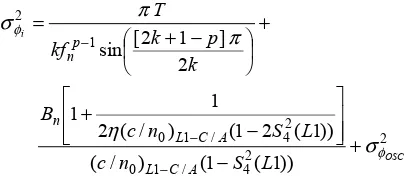
Finally, from the equation 7, 8 and 9, the phase tracking error variance (rad2) at the output of L1 carrier PLL including scintillation and thermal noise is given as:

2 2 4 / 1 0 2 4 / 1 0 1 2 )) 1 ( 1 ( ) / ( )) 1 ( 2 1 ( ) / ( 2 1 1 2 ] 1 2 [ sin OSC i L S n c L S n c B k p k kf T A C L A C L n p n φ φ σ η π π σ + − ⎥ ⎥ ⎦ ⎤ ⎢ ⎢ ⎣ ⎡ − + + ⎟ ⎠ ⎞ ⎜ ⎝ ⎛ + − = − − − (10)

which is valid provided 1< p<2k.

IV. RESULTS AND ANALYSES

The experiments in this paper were based on set from receiving stations Longyearbyen (LYB0) with coordinate 78.2°N, 16.0°E and Ny Alesund (NYA1) with coordinate 78.9°N, 11.9°E, which have a baseline ~ 125 km, for the time period 2000 – 2300 UT, 10th Dec 2006. The accuracy for baseline computation based on a conventional ‘non-mitigated’ or ‘equal weights’ solution is compared against a ‘mitigated’ solution using the approach which defines the observable variances based on the tracking errors variance as described in (i) Section III and, (ii) elevation angles.

[image:3.595.308.510.239.329.2]

The standard deviations adopted for the different observables in the standard case (non-mitigated where all satellites observations are assumed to be independent and their qualities of measurement are the same) are shown in Table I.

TABLE I. OBSERVABLE STANDARD DEVIATIONS ADOPTED FOR THE

STANDARD CASE (NON-MITIGATED)

Observable standard deviations Values (m)

CA

σ for C/A observable 0.600

2

P

σ for P2 observable 0.800

1

L

φ

σ for L1 observable 0.006

2

L

φ

[image:4.595.63.287.61.236.2] [image:4.595.320.544.113.375.2]

Figure 1. S4 (upper panel) and σ_φ (lower panel) measured at station NYA1 (20 – 23 UT, 10th _{Dec 2006).}

Figure 2. S4 (upper panel) and σ_φ (lower panel) measured at station LYB0 (20 – 23 UT, 10th _{Dec 2006).}

Figures 1 and 2 show the time series of amplitude and phase scintillation indices, respectively S4 and σφ for all available satellites above the elevation angle of 10o at stations NYA1 (rover station) and LYB0 (base station)

Figures 3 and 4 show the time series for the height and 3D errors (height + horizontal errors) estimated at the station NYA1, for both the non-mitigated (standard stochastic model as described in TABLE I) and the mitigated approach using tracking error variances and elevation angles as weighting parameters in modified stochastic model.

From the time series shown in Figures 3 and 4, it is apparent that the positioning accuracy has been improved when the scintillation mitigation approach is applied. There is more than 11% improvement for the average height errors during this 3 hour data period and more than 10% improvement in the 3D positioning error when tracking error variances were used as weighting parameters in a modified stochastic model.

However, there is more than 10% improvement for the average height errors and more than 8% improvement in the 3D positioning error when elevation angles were used as weighting parameters in a modified stochastic model. A summary of the results is given in Table II.

Figure 3. Height error for the non-mitigated (upper panel), the mitigated solution using tracking error variances (center panel) and elevation angles

[image:4.595.63.287.293.466.2]

(bottom panel) at station NYA1

Figure 4. 3D error for the non-mitigated (upper panel), the mitigated solution using tracking error variances (center panel) and elevation angles (lower

panel) at station NYA1

0 20 40 60 80 100 120 140 160 180

0 0.2 0.4 0.6 0.8

Time (minutes)

S4

0 20 40 60 80 100 120 140 160 180

0 0.1 0.2 0.3 0.4

Time (minutes)

Ph

i6

0

0 20 40 60 80 100 120 140 160 180

0 0.2 0.4 0.6 0.8

Time (minutes)

S4

0 20 40 60 80 100 120 140 160 180

0 0.1 0.2 0.3 0.4

Time (minutes)

Ph

i6

[image:4.595.320.541.414.682.2]

TABLE II. SUMMARY OF THE STATIC POSITIONING.

Non-mitigated

Mitigated Improvement (%)

Tracking error variance

Elevation angle

Tracking error variance

Elevation angle

RMS height error (m)

0.843792 0.746611 0.756846 11.52 10.304

RMS 3D error (m)

0.922785 0.825548 0.843588 10.537 8.582

V. CONCLUSION

In this section, a modified stochastic model was used to enable different weighting algorithms to be used in a least squares adjustment. There are two different types of weighting models that were considered to investigate their potential positioning improvement for ionospheric effects, viz. (i) tracking error variances in the receiver; and (ii) elevation angle. Using tracking error variances and elevation angles as weighting models have shown some improvement in positioning accuracy with particular data set. Based on our studies and analysis of particular data sets, using tracking error variances as a weighting model shows the most improvement for GPS positioning (as large as 11% in height error and 10% in 3D error).

ACKNOWLEDGMENT

The authors would like to acknowledge Dr. Vincenzo Romano and colleagues at Istituto Nazionale di Geofisica e Vulcanologia (INGV) for the provision of the GPS data from Longyearbyen and Ny Alesund in Svalbard.

REFERENCES

[1] R. S. Conker, M. B. El-Arini, C. J. Hegarty, and T. Hsiao, Modelling the Effects of Ionospheric Scintillation on GPS/Satellite-Based Augmentation System Availability. Radio Sci., 38, 1, 1001, doi: 10.1029/2000RS002604.2003.

[2] C. C. J. M. Tiberius, N. Jonkman, and F. Kenselaar, The Stochastics Of

GPS Observables, GPS World, 10, 2, 49-54, 1999J. Clerk Maxwell, A Treatise on Electricity and Magnetism, 3rd ed., vol. 2. Oxford: Clarendon, 1892, pp.68–73.

[3] M. Knight, A. Finn, The Effects Of The Ionospheric Scintillation On

GPS, paper presented at ION-GPS-1998, Inst. Of Navigation, Nashville, Tenn., 15 – 18 Sept 1998

[4] C. J. Hegarty, Analytical Derivation Of Maximum Tolerable In-Band