Published online 16 September 2005 in Wiley InterScience (www.interscience.wiley.com). DOI: 10.1002/mrc.1674
Analysis and elimination of artifacts in indirect
covariance NMR spectra via unsymmetrical processing
Kirill A. Blinov,
1Nicolay I. Larin,
1Mikhail P. Kvasha,
1Arvin Moser,
2Antony J. Williams
2and
Gary E. Martin
3∗1Advanced Chemistry Development, Moscow Department 6 Akademik Bakulev Street, Moscow 117512 Russian Federation, Russia 2Advanced Chemistry Development 110 Yonge Street 14th Floor Toronto M5C 1T4, Ontario Canada
3Pfizer Global Research and Development Analytical Research and Development 7000 Portage Road Kalamazoo, Michigan 49001-0199, USA
Received 8 May 2005; Revised 27 June 2005; Accepted 29 June 2005
Indirect covariance NMR offers an alternative method of extracting spin–spin connectivity information via the conversion of an indirect-detection heteronuclear shift-correlation data matrix to a homonuclear data matrix. Using an IDR (inverted direct response)-HSQC-TOCSY spectrum as a starting point for the indirect covariance processing, a spectrum that can be described as a carbon–carbon COSY experiment is obtained.
These data are analogous to the autocorrelated 13C–13C double quantum INADEQUATE experiment
except that the indirect covariance NMR spectrum establishes carbon–carbon connectivities only between contiguous protonated carbons. Cyclopentafuranone and the complex polynuclear heteroaromatic
naphtho[2′,1′:5,6]-naphtho[2′,1′:4,5]thieno[2,3-c]quinoline are used as model compounds. The former is a
straightforward example because of its well-resolved proton spectrum, while the latter, which has considerable resonance overlap in its congested proton spectrum, gives rise to two types of artifact
responses that must be considered when using the indirect covariance NMR method. Copyright2005
John Wiley & Sons, Ltd.
KEYWORDS:indirect covariance NMR; IDR-HSQC-TOCSY; carbon–carbon vicinal correlation
INTRODUCTION
There have been several recently published reports that have outlined the principles behind covariance NMR spectroscopy.1,2More recently, Br ¨uschweiler and coworkers described covariance NMR spectroscopy by singular value decomposition for homonuclear 2D NMR data3 in addition to indirect covariance NMR spectroscopy for use on het-eronuclear 2D NMR data.4The latter method was of interest in that it provides the means of obtaining homonuclear 2D NMR spectra of the insensitive nucleus of a heteronuclide pair with detection via the sensitive nuclide. Beginning with an HSQC-TOCSY data set, the resulting indirect covari-ance NMR spectrum is the equivalent of an autocorrelated 13C–13C double quantum INADEQUATE spectrum.5 – 8
How-ever, unlike the autocorrelated INADEQUATE spectrum, which affords correlations between both protonated and quaternary carbon resonances, the indirect covariance NMR spectrum is more accurately described as a protonated car-bon CC-COSY spectrum and is only capable of furnishing connectivity information between contiguous protonated carbons.
To explore this new method, we elected to use data sets for several model compounds, which included
ŁCorrespondence to: Gary E. Martin, Analytical R & D
0200/259/277, Pfizer Global Research & Development, 7000 Portage Road, Kalamazoo, MI 49001-0199, USA.
E-mail: [email protected]
the cyclopentafuranone (1, (3aR,4S,5R,6aS )-5-hydroxy-4-(hydroxymethyl)hexahydro-2H-cyclopenta[b]furan-2-one) and the complex polynuclear aromatic heterocycle naphtho [20
,10
:5,6]naphtho[20
,10
covariance NMR spectra
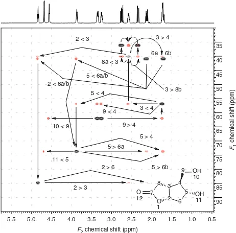
The annotated IDR (inverted direct response)-HSQC-TOCSY spectrum of cyclopentafuranone (1) is shown in Fig. 1. Direct correlation responses correspond exactly to the correlations of an HSQC spectrum and are inverted by the pulse sequence used.9,10Negatively phased direct correlation responses are represented by black contours in Fig. 1. Relayed correlation responses have a positive phase and are defined by red contours. The mixing time used during the acquisition of these data was 18 ms. The relatively short mixing time provided coherence transfer to only vicinal neighbor protons almost exclusively. Variations in the relayed response intensity observed in Fig. 1 are a function of the size of the vicinal coupling constant between the correlated protons through which coherence was transferred.
The indirect covariance NMR spectrum of1obtained by processing the IDR-HSQC-TOCSY frequency domain spec-trum according to the method of Zhang and Br ¨uschweiler4 is shown in Fig. 2. The well-resolved proton spectrum of1, which has only a single pair of overlapping proton reso-nances, yields an indirect covariance NMR spectrum that is straightforward to interpret and assign. The anisochronous C9 methylene resonance at 61.9 ppm provides a convenient starting point for the assignment of both the HSQC-TOCSY spectrum in Fig. 1 as well as the indirect covariance NMR spectrum shown in Fig. 2. The negative off-diagonal response
5.5 5.0 4.5 4.0 3.5 3.0 2.5 2.0 1.5 1.0 0.5
F2 chemical shift (ppm)
35
chemical shift (ppm)
9 > 4
Figure 1.Inverted direct response HSQC-TOCSY spectrum of cyclopentafuranone (1) acquired with an 18-ms mixing time. Proton– carbon direct correlation responses have negative phase and are denoted by black contours; relayed coherence responses have a positive phase and are denoted by red contours. The numbering scheme used is shown by the structure inset. Responses are labeled using the convention of listing the downfield resonance followed by the upfield resonance.
to C5 are much weaker than the C4–C9 correlation as a con-sequence of the small vicinal proton couplings to H4 (see the proton reference spectrum plotted above the HSQC-TOCSY spectrum in Fig. 1). Correlations linking C5 to C6 and C3 to C8 (labeled C6–C5 and C8–C3, respectively) are consider-ably more intense. Finally, the correlations linking both C6 and C3 to C2 are only partially resolved and are again weak because of small vicinal proton–proton couplings.
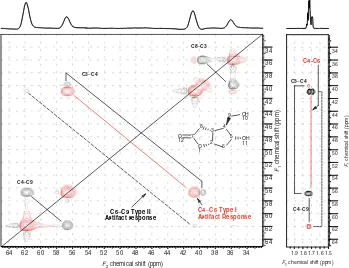
The indirect covariance NMR spectrum shown in Fig. 2 also contains a pair of prominent positive off-diagonal responses labeled as the C4–C6 Type I artifact response. We have found that when using IDR-HSQC-TOCSY spectra such as that shown in Fig. 1 for indirect covariance NMR processing, two types of artifacts are observable due to proton-resonance overlap. Zhang and Br ¨uschweiler4referred to artifacts because of proton resonance overlap in general terms but did not elaborate further on this aspect of indirect covariance NMR spectra. Figure 3 shows a side-by-side presentation of the upfield region of the indirect covariance spectrum shown in Fig. 2 with the appropriate segment of the HSQC-TOCSY spectrum from Fig. 1. Note that in the right panel of Fig. 3, there are two IDRs corresponding to H4–C4 and H6b–C6. Relayed coherence responses are also observed from H3 ! H4 at the chemical shift of C3 and from H9 ! H4 at the chemical shift of C9. The pair of correlations in the right panel for the H4/C4 direct response
C4−C6 Type I Artifact response
90 85 80 75 70 65 60 55 50 45 40 35 30
F2 chemical shift (ppm)
35
chemical shift (ppm)
C2 C5
Figure 2.Indirect covariance NMR spectrum of
C4−C6 Type I
Artifact Response
C4-C6
1.9 1.8 1.7 1.6 1.5
F
2 chemical shift (ppm)
34
chemical shift (ppm)
64 62 60 58 56 54 52 50 48 46 44 42 40 38 36 34 F2 chemical shift (ppm)
34
chemical shift (ppm)
7
Figure 3.Composite presentation of a segment of the indirect covariance NMR spectrum (left panel) and the corresponding region of the HSQC-TOCSY spectrum (right panel). Relative to the spectrum shown in Fig. 2, the threshold for the lowest contour is somewhat lower. The positive off-diagonal correlations in the left panel labeled C4– C6 Type I artifact response arise owing to the overlap of the H4 and H6 protons in the data from the HSQC-TOCSY spectrum as shown in both panels connected by a solid red line. The very weak pair of correlations in the left panel connected by the dashed black line labeled C6– C9 Type II artifact again arises as a consequence of the overlap of H4 and H6. The direct response from H6b at the chemical shift of C6 and the relayed response from the C9 methylene resonances to H4 at the chemical shift of C9 give rise to the negative-phase off-diagonal Type II artifact responses. A slightly deeper threshold level was used when plotting the data shown in this figurevsthe data shown in Fig. 2,
allowing the Type II response to be observed.
and the relayed H3!H4/C3 response gives rise to the weak C3–C4 vicinal carbon–carbon correlation response in the left panel as expected in the indirect covariance NMR spectrum. A second pair of responses for the H4/C4 direct response and the relayed H9 ! H4 response at the C9 chemical shift affords the C4–C9 vicinal carbon–carbon correlation response, as expected.
The positive-phase off-diagonal responses in the indirect covariance spectrum arise because of H4/H6b proton-resonance overlap; the direct responses for H6b/C6 and H4/C4 connected by the solid red line in the right panel define this correlation, which we have elected to label as a Type I artifact. The positive phase of this type of artifact response makes it possible to visually eliminate them from consideration when interpreting any indirect covariance NMR spectrum. Type I artifact responses can arise between a pair of IDRs as in this case or between a pair of positive-phase relayed coherence responses (see the discussion of the indirect covariance NMR spectrum of naphtho[20
,10
:5,6]naphtho[20
,10
:4,5]thieno[2,3-c]quinoline (2) later). In both cases, the responses in the indirect covariance for these artifacts have a positive phase. It is also worth noting at this point that when conventional HSQC-TOCSY data, rather than IDR-HSQC-TOCSY data, are subjected to indirect covariance processing, all responses in the spectrum have the same phase (positive) rendering the Type I artifacts
indistinguishable from any other response in the spectrum, thereby further complicating the interpretation of the data.
The weak, negative-phase off-diagonal response in the indirect covariance spectrum shown in the left panel of Fig. 3 and labeled C6–C9 Type II artifact response arises because of the IDR for H6b/C6 and the positive-phase relayed response for H9 ! H4 at the C9 chemical shift. This pair of responses gives rise to a very weak negative-phase off-diagonal response in the indirect covariance NMR spectrum that looks like a legitimate vicinal carbon–carbon correlation response. The response, however, is a type of artifact response that we have labeled Type II. This type of artifact response is indistinguishable from the carbon–carbon vicinal correlation responses sought in the experiment, and thus represents, in our opinion, a shortcoming of the method. While the single Type II response visible in the indirect covariance NMR spectra shown in Figs 2 and 3 is very weak and thus of little concern, similar Type II responses observed in the indirect covariance NMR spectrum of naphtho[20
,10
:5,6]-naphtho[20
,10
:4,5]thieno[2,3-c]quinoline (2) have intensity comparable to the legitimate carbon–carbon vicinal connectivity correlations and are thus more problematic.
of the artifact responses will have identical phases since all of the responses in the spectrum are positive. Hence Type I artifact responses will be indistinguishable from Type II artifact responses or from legitimate carbon–carbon vicinal correlation responses. In this regard, it is preferable to utilize IDR-HSQC-TOCSY when indirect covariance processing is contemplated. The use of HSQC rather than the HMQC-based variant of the experiment is also preferable HMQC-based on the improved F1 resolution of the former, which is comparable to the difference in F1 resolution between an HMQC and HSQC experiment.11
Moving from cyclopentafuranone (1) to naphtho[20
,10
: 5,6]naphtho[20
,10
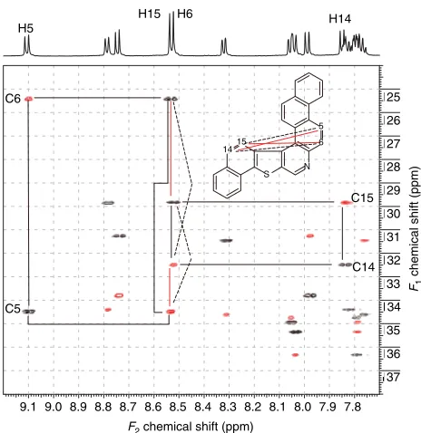
:4,5]-thieno[2,3-c]quinoline (2), which has a much more complex and overlapped proton spectrum even at 600 MHz, as expected, both the IDR-HSQC-TOCSY and indirect covariance NMR spectra are con-siderably more complex. The IDR-HSQC-TOCSY spec-trum of 2 is shown in Fig. 4. The total assignment of 2, based on the use of IDR-HSQC-TOCSY data, has been reported.11,12 For purposes of a discussion of the indi-rect covariance NMR spectrum of 2, we will focus on two isolated two-spin systems, H5/C5–H6/C6 (9.09/134.4 and 8.52/125.4 ppm, respectively) and H14/C14–H15/C15 (7.84/132.5 and 8.53/129.8 ppm, respectively). As would be expected from the overlap of H6 and H15 resonating at 8.52 and 8.53 ppm, respectively, 2has considerable poten-tial for the observation of artifact responses in the indirect covariance NMR spectrum. The location of the two-spin systems on which the discussion of the indirect covari-ance NMR spectrum will be based is shown by 3. The desired vicinal carbon–carbon correlations are denoted in the structure by the solid black lines. From the analysis of the indirect covariance NMR spectrum of 2 shown in Fig. 5, the solid red and dashed black lines, correspond-ing to Type I and Type II artifacts, respectively, are also shown. It is important to note that the lines signifying the resonances leading to Type II artifacts cannot be drawn in arbitrarily; the spectrum must be analyzed to deter-mine which resonances are associated with Type II artifact responses.
S 15 14
N 6 5
3
9.1 9.0 8.9 8.8 8.7 8.6 8.5 8.4 8.3 8.2 8.1 8.0 7.9 7.8 F2 chemical shift (ppm)
125
126
127
128
129
130
131
132
133
134
135
136
137 F1
chemical shift (ppm)
S 15 14
N 6 5 C6
C5
C15
C14
Figure 4.IDR-HSQC-TOCSY spectrum of
naphtho[20,10:5,6]naphtho[20,10:4,5]-thieno[2,3-c]quinoline (2). Correlation pathways for the H5/C5– H6/C6 and
H14/C14– H15/C15 resonant pairs are shown. The H6 and H15 protons, which resonate at 8.52 and 8.53 ppm, respectively, correspond to the completely overlapped ‘doublet’ centered at ¾8.255 ppm. As a consequence of the overlap of these proton
resonances, both Type I and Type II artifact responses are expected in the indirect covariance NMR spectrum of2. Artifact responses will also be expected for the overlapped proton resonances near 8.05 and 7.80 ppm.
136 135 134 133 132 131 130 129 128 127 126 125
F2 chemical shift (ppm)
125
chemical shift (ppm)
C6–C5
Figure 5.Indirect covariance NMR spectrum of naphtho[20
,10
:5,6]naphtha-[20 ,10
:4,5]thieno[2,3-c]quinoline (2).
The data were processed according to the method of Zhang and Br ¨uschweiler.3Connectivities are shown for the C5– C6 and C14– C15 spin systems whose correlation pathways are defined in the IDR-HSQC-TOCSY spectrum shown in Fig. 4. The expected vicinal carbon– carbon connectivities between C5– C6 and C14– C15 are denoted by off-diagonal correlations linked by solid black lines. The vicinal carbon– carbon
correlation for C3– C4 (solid black line) overlaps the Type II C15– C13 and C15– C5 artifact responses (dashed black line) in the spectrum. The Type II artifact response labeled C6– C14 and the two Type I artifact responses labeled C6– C15 and C14– C5 (denoted by solid red lines) are resolved and do not represent multiple responses.
the data without broadband 13C decoupling during the acquisition period. In the resulting coupled HXQC-TOCSY or -ROESY spectrum [X D M (multiple) or D S (single)], the direct responses are displaced by š⊲1J
CH⊳/2, allow-ing the relayed responses to be observed. Several reports in the literature have used this approach successfully for HMQC-TOCSY13 and HMQC-ROESY.14 The other alterna-tive is to completely suppress the direct responses using the SDR (suppressed direct response)-HSQC-TOCSY pulse sequence.15 Rather than using a pulse sequence element comprising 180° pulses applied to both proton and carbon
as in the IDR experiment, the SDR variant of the exper-iment applies a 90°, 1H pulse and a 180°, 13C pulse to completely suppress the direct response. Either of these approaches can presumably establish the H2/C2–H3/C3 correlation. However, in the former case, calculation of the indirect covariance NMR spectrum from a 13C cou-pled HSQC-TOCSY experiment can produce only artifact responses because of resonance overlap. In the case of the SDR-HSQC-TOCSY spectrum, an indirect covariance NMR spectrum cannot be calculated as there will be, in princi-ple, only the relayed response at any given proton chemical shift.
136.5 136.0 135.5 135.0 134.5 134.0 133.5 133.0 132.5 132.0 131.5 131.0 130.5 130.0
F2 chemical shift (ppm)
129.5
chemical shift (ppm)
C15
12–15 14–15 16 15
17–16
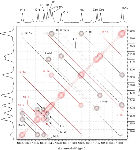
Figure 6.Annotated expansion of the indirect covariance NMR spectrum of naphtho[20,10:5,6]naphtho[20,10:4,5]
thieno[2,3-c]quinoline (2) shown in Fig. 5. Legitimate
carbon– carbon vicinal correlations are denoted by solid black lines. Type I artifact responses are denoted by solid red lines. Type II artifact responses are denoted by dashed black lines. A 13C reference spectrum processed with 10-Hz exponential
broadening is plotted above the contour plot; a projection through theF1frequency domain is plotted along the left side
of the contour plot. Volume integration of the peaks in the indirect covariance spectrum was used to determine the overlap of the 3– 4 carbon– carbon vicinal correlation response (solid black line) with the Type II artifact responses labeled 15– 3 and 15– 5 (dashed black line).
As expected from the analysis of the IDR-HSQC-TOCSY spectrum shown in Fig. 4, a pair of Type I responses is observed in the indirect covariance NMR spectrum shown in Fig. 5 between C5–C14 and C6–C15. These are denoted in Fig. 5 by solid red lines. The Type I artifact responses arise from a pair of either direct or relayed responses from different spin systems as denoted by the solid red lines shown for the strongly overlapped H15/H16 resonances in F2 in Fig. 4. In addition, multiple Type II responses are observed in Fig. 5 between the C15–C3, C15–C5, and C6–C14 resonant pairs, these correlations are denoted by dashed black lines. The Type II artifact responses arise for a direct and relayed response, again from different spin systems, as defined by the dashed black lines at the F2 frequency of the overlapped H15/H16 resonances in Fig. 4. A vicinal correlation response between C3 and C4 overlaps the Type II C15–C3 and C15–C5 artifact responses and is denoted by the solid black line in Fig. 5.
Type II artifacts arise from a negatively phased, direct and a positively phased relay response, albeit from dif-ferent spin systems, they will have positive phase, and there is no convenient means of visually identifying these responses in a conventional indirect covariance spec-trum other than through the analysis of the specspec-trum. We will demonstrate, however, that these responses can be manipulated and subsequently eliminated through a modification of the indirect covariance–processing proto-col described later followed by symmetrization as used with diagonally symmetric spectra such as COSY and TOCSY.
One other point is worth considering if we assume that the transfer efficiency during the isotropic mixing period is identical for all of the relayed coherence trans-fer responses in an HSQC-TOCSY spectrum. This will only be approximately valid in a case such as that rep-resented by 2when all of the vicinal proton–proton cou-pling constants are more or less identical. In such a case, Type II artifact responses, which arise only once in a spectrum, e.g. the response for C6–C15 (125.4–129.7 ppm in Fig. 6), will have only half of the observed response intensity of a legitimate carbon–carbon vicinal correlation response, e.g. C5–C6 (134.5–125.4 ppm in Fig. 6), in the indi-rect covariance spectrum. This statement is based on the observation that the C5–C6 vicinal carbon–carbon corre-lation responses in the indirect covariance spectrum arise from the pairs of direct and vicinal relayed responses observed at the proton frequencies of both H5 and H6 in the F2 frequency domain. This observation was con-firmed for the indirect covariance spectrum of 2 shown in Fig. 6 by volume integration of the responses in the data matrix.
The more complex and congested downfield region of the indirect covariance NMR spectrum of2is presented in Fig. 6. The correlations are denoted by the same convention used in Fig. 5. To illustrate the distribution of Type I and II artifact responses relative to the structure of the molecule, all of the artifact correlations observed in Figs 5 and 6 are collected on 4. The expected carbon–carbon vicinal correlation responses between contiguous protonated carbons are not shown. Although the total number of artifact responses might initially be assumed to render indirect covariance NMR undesirable, it should be kept in mind that all of the Type I artifact responses can be ignored on simple visual inspection of the data matrix. There are only a total of five Type II artifact responses contained in data shown in Figs 5 and 6. Four of the Type II artifacts have response intensity that makes them indistinguishable from authentic carbon–carbon vicinal correlation responses by casual visual inspection. Since the vicinal proton–proton coupling constants are relatively uniform in a molecule such as 2, the Type II artifact responses are, however, distinguishable based on volume integration as discussed above.
S 15 14
10 11 13
12
8 N
6 5 16
17
4 3 2 1
134.9 134.4
129.8
134.5
125.4
144.4 135.3
136.3
134.6
131.4 132.5
129.7
131.2
4
Elimination of artifact responses through
unsymmetrical covariance processing
The phase characteristics of the responses contained in the IDR-HSQC-TOCSY spectrum allow the direct (negative phase) and relayed or TOCSY responses (positive phase) to be considered separately. Hence, as shown schematically in Fig. 7, the IDR-HSQC-TOCSY spectrum can be decomposed into a pair of data matrices, one containing only the negative-phase direct responses and the other the positive-negative-phase relayed or TOCSY responses. After decomposition of the IDR-HSQC-TOCSY spectrum into a positive- and negative-phase matrix, the pair of matrices can be subjected to the covariance procedure according to the following scheme. In the usual covariance-processing protocol, diagonally symmetric peaks arise from equal rows:
RowIðRowJ and RowJðRowI
In the modified covariance procedure proposed in this work, diagonally symmetric peaks arise from different rows in the fashion:
⊲C⊳RowIð⊲⊳RowJ
and
⊲C⊳RowJð⊲⊳RowI
This process is shown schematically in Fig. 8. When the process is repeated for the other pair of responses that comprise the usual pattern of responses in an IDR-HSQC-TOCSY spectrum, the intensity of the diagonally symmetric responses is effectively doubled (assuming equivalent cou-pling constants and efficiency of magnetization transfer during the mixing period).
IDR-HSQC-TOCSY data matrix
Row I
Row J Positive matrix (relayed responses)
Negative matrix (direct) Direct responses Relayed or
TOCSY responses (positive)
Row I
Row J Row I
Row J
Figure 7.Schematic representation of the decomposition of an IDR-HSQC-TOCSY data matrix into a positive and negative matrix based on response phase. Inverted direct responses are collected in the negative matrix while the TOCSY or relayed responses are collected in the positive matrix.
Row I Positive matrix
(long-range)
Row j
Row I Negative matrix
(direct)
Row j
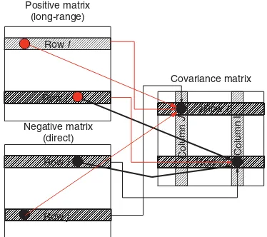
Covariance matrix
zRow I
Column
J
Column I
Row J
Figure 8.Schematic representation of the covariance processing of an IDR-HSQC-TOCSY spectrum decomposed into positive (TOCSY or relayed responses) and negative (direct correlation responses) data matrices. For a vicinally coupled pair of resonances in the IDR-HSQC-TOCSY spectrum, e.g. represented by the H5/C6, H5/C5, H6/C6 and H6/C5 responses in Fig. 4, the diagonal carbon– carbon correlation response arises as shown above from the multiplication of
⊲C⊳RowIð⊲⊳RowJand⊲C⊳RowJð⊲⊳RowI. The phase of
the diagonally symmetric carbon– carbon vicinal correlation response is negative, denoted by the black responses in the covariance matrix on the right.
responses as in the case of a legitimate carbon–carbon vicinal correlation response. This result is shown schematically in Fig. 9.
To illustrate what we have shown schematically in Figs 7–9, the IDR-HSQC-TOCSY data set presented in Fig. 4 was used as an example. To simplify the presentation for purposes of this discussion, all of the responses in the
Row I Positive matrix
(long-range)
Row J
Row I Negative matrix
(direct)
Row J
Covariance matrix
Row I
Column
J
Column
I
Row J
Figure 9.Schematic representation of the behavior of artifact responses during covariance processing. The positive and negative-phase responses that would give rise to a Type II occur only at the proton shift in what would correspond to column I. When the corresponding rows are multiplied,
⊲C⊳RowIð⊲⊳RowJ, a single response is produced in the
resulting covariance matrix at the intersection of RowIand
ColumnJ. There is no diagonally symmetric response as in the
case of a legitimate carbon– carbon vicinal correlation response shown schematically in Fig. 8.
data matrix except for those responsible for causing the appearance of artifact responses in Fig. 5 were replaced by noise taken from a random location on the noise floor of the data matrix. The correspondingly modified IDR-HSQC-TOCSY data matrix is shown in the left panel of Fig. 10. When these data are subjected to the covariance procedure, the resulting data matrix is shown in the right panel of Fig. 10. Legitimate carbon–carbon vicinal correlation responses are diagonally symmetric as expected. Artifact responses are diagonally asymmetric and lend themselves to removal by the symmetrization routine that has been used for many years with COSY spectra. When the full IDR-HSQC-TOCSY data matrix shown in Fig. 4 is subjected to the covariance-processing protocol shown schematically in Figs 7–9, the resulting spectrum is shown in Fig. 11.
CONCLUSIONS
9.0 8.5 8.0 F2 chemical shift (ppm)
124
126
128
130
132
134
136 F1
chemical shift (ppm)
134 132 130 128 126
F2 chemical shift (ppm)
125
126
127
128
129
130
131
132
133
134 F1
chemical shift (ppm)
Artifact responses (asymmetric)
Figure 10.The IDR-HSQC-TOCSY spectrum of2is shown in the left panel. All of the responses in the data matrix except for those responsible for the artifacts observed in Fig. 5 have been replaced by noise taken from a random location on the noise floor of the spectrum. By subjecting the data matrix on the left to decomposition, as shown schematically in Fig. 7, followed by covariance processing as illustrated schematically in Figs 8 and 9, the data matrix shown in the right panel is the indirect covariance result of the manipulation. The asymmetric nature of the Type II artifact responses allows their removal by simple symmetrization of the type used with homonuclear COSY data.
136 135 134 133 132 131 130 129 128 127 126 125
F2 chemical shift (ppm)
124
125
126
127
128
129
130
131
132
133
134
135
136
137
F1
chemical shift (ppm)
C6–C5
C15–C14 C4–C3
Figure 11.When the full IDR-HSQC-TOCSY spectrum of2
shown in Fig. 4 is subjected to the processing scheme illustrated by Figs 7– 9, the experimental result is shown above. Correlations for three vicinal carbon– carbon correlations are denoted by solid black lines. Two of these correspond to the C5– C6 and C14– C15 correlations. The other arises from the C3– C4 correlation and is shown because one of the correlations from this diagonally symmetric pair overlaps the Type II artifact response that was shown in the right panel of Fig. 10. A 10-Hz broadened13C reference spectrum is plotted above the contour plot to provide a better representation of the position of all of the carbon resonances in the spectrum of2.
correlations and can only be differentiated from the latter by the analysis of the indirect covariance spectrum in par-allel with the IDR-HSQC-TOCSY data or through volume integration in the particular case when all of the vicinal pro-ton–proton homonuclear couplings are nearly identical as in the case of a polynuclear aromatic or heteroaromatic such as
2. In the congested region of the13C spectrum of IDR-HSQC-TOCSY spectrum of 2 ranging from about 133–137 ppm, the indirect covariance NMR spectrum (compare Figs 4 and 6) may offer some advantages over the IDR-HSQC-TOCSY spectrum in terms of interpretability, although the issue of Type II artifact responses must be considered.
In the second half of the present study, we have shown that a modified or unsymmetrical covariance-processing scheme applied to IDR-HSQC-TOCSY data can be used in conjunction with symmetrization to remove artifacts from indirect covariance NMR spectra, thereby eliminating ambiguities that could arise in the interpretation of these data when dealing with an unknown chemical structure. This approach should allow the indirect covariance method to be applied to a diverse range of organic molecules including molecules of considerable complexity.
carbon–carbon connectivities, including partial substruc-tures extracted from this approach, can reduce the challenge of generating resultant structures from the CASE system, which is presently being evaluated. The removal of the artifacts using the unsymmetrical covariance–processing scheme discussed in this work precludes using potentially incorrect carbon–carbon connectivity information in the data input matrix for a CASE program and further helps in improving the utility of this approach to novel chemical structure determination.
EXPERIMENTAL
The sample of cyclopentafuranone (1) was obtained from Sigma–Aldrich. The sample of 2 used in this study was synthetically prepared.11,12Samples were prepared for NMR data acquisition by dissolving¾5 mg of each compound in deuterochloroform in a 3-mm NMR tube.
NMR experiments performed on 1 used a Varian Inova 500 MHz NMR; experiments performed on 2 used a Varian Inova 600 MHz spectrometer. Both instruments were equipped with 3 mm Nalorac micro inverse detection gradient NMR probes. A mixing time of 18 ms was used to acquire the IDR-HSQC-TOCSY spectra of both1and2
shown in Figs 1 and 4, respectively. The IDR-HSQC-TOCSY spectrum of1was acquired using 512 points inF2 with 96 increments of the evolution time, t1. Data were processed by zero-filling to 1024 in t2 and linear predicting from 96 to 128 points followed by zero-filling to 256 points in the second time domain. Gaussian multiplication was used in both time domains. The IDR-HSQC-TOCSY spectrum of2
was acquired as 512 points int2and again zero-filled to 1024 points; the experiment was digitized with 160 increments of the evolution time,t1, in the second frequency domain; the data were linear predicted to 256 points and zero-filled to 512 points inF1during processing. Gaussian multiplication was used in both time domains.
The indirect covariance NMR spectra were computed with the method of Zhang and Br ¨uschweiler,4 using the 2D NMR Manager module of ACD/SpecManager23 v8.2. The processing was performed using a PC with a 2.8 GHz Pentium IV processor with 1 Gbyte of RAM. The calculation of the indirect covariance NMR spectra from the processed IDR-HSQC-TOCSY data took approximately 4 s.
REFERENCES
1. Br ¨uschweiler R, Zhang F.J. Chem. Phys.2004;120: 5253. 2. Br ¨uschweiler R.J. Chem. Phys.2004;121: 409.
3. Trbovic N, Smirnov S, Zhang F, Br ¨uschweiler R.J. Magn. Reson. 2004;171: 277.
4. Zhang F, Br ¨uschweiler R.J. Am. Chem. Soc.2004;126: 13 180. 5. Turner DL.Mol. Phys.1981;44: 1051.
6. Turner DL.J. Magn. Reson.1982;49: 175. 7. Turner DL.J. Magn. Reson.1983;53: 259.
8. Musmar MJ, Willcott MR III, Martin GE, Gampe RT Jr, Iwao M, Lee ML, Hurd RE, Johnson LF, Castle RN.J. Heterocycl. Chem. 1983;20: 1661.
9. Domke T.J. Magn. Reson.1991;95: 174.
10. Crouch RC, Davis AO, Martin GE.Magn. Reson. Chem.1995;33: 889.
11. Hadden CE, Martin GE, Luo J-K, Castle RN.J. Heterocycl. Chem. 1999;36: 533.
12. Hadden CE, Martin GE, Luo J-K, Castle RN.J. Heterocycl. Chem. 2000;37: 821.
13. Crouch RC, McFadyen RB, Daluge SM, Martin GE.Magn. Reson. Chem.1990;28: 792.
14. Kawabata J, Fukushi E, Mizutani J.J. Am. Chem. Soc.1992;114: 1115.
15. Martin GE, Spitzer TD, Crouch RC, Luo J-K, Castle RN. J. Heterocycl. Chem.1992;29: 577.
16. Martin GE. Cryogenic NMR probes: applications. InEncyclopedia of Nuclear Magnetic Resonance, Vol. 9: Advances in NMR, Grant DM, Harris RK (eds). Wiley: Chichester, 2002; 33. 17. Martin GE. Applications of cryogenic NMR probe technology
for the identification of low-level impurities in pharmaceuticals. In Handbook of Modern Magnetic Resonance, vol. 2, Craik DJ, Webb GA (eds). Elsevier: Amsterdam, 2005.
18. Martin GE. Small volume and high sensitivity NMR probes. In Ann. Report NMR Spectrosc., vol. 56, Webb GA (ed). Elsevier: Amsterdam, 2005.
19. Blinov KA, Carlson D, Elyashberg ME, Martin GE, Mar-tirosian ER, Molodtsov SG, Williams AJ. Magn. Reson. Chem. 2003;41: 359.
20. Elyashberg ME, Blinov KA, Martirosian ER, Molodtsov SG, Williams AJ, Martin GE.J. Heterocycl. Chem.2003;40: 1017. 21. Elyashberg ME, Blino KA, Molodtsov SG, Williams AJ,
Martin GE.J. Chem. Inf. Comput. Sci.2004;44: 771.
22. Molodtsov SG, Elyashberg ME, Blinov KA, Williams AJ, Martin GE.J. Chem. Inf. Comput. Sci.2004;44: 1737.