On-Load Tap Classification using
Supervised Learning on Reg-D Transformer
Data
⋆
J du Toit∗
∗
Eskom Distribution, Western Cape Operating Unit, Eskom road, Brackenfell, South Africa (Tel: +27 (0)21 980 3915; e-mail:
Abstract:The goal of this study was to explore the possibility of creating a statistical model
of a live 66kV-11kV 20MVA transformer, in an effort to validate the significance of recently accumulated Reg-D relay substation data, in enabling power system monitoring by means of predictive analytics. Power transformer data was obtained from a live substation over a period of one month, and used to develop a model with which to predict the transformer’s mechanical tap position. Both multi-class logistic regression and artificial neural network methodologies were implemented, tested, and the results compared. Results indicate a significant performance advantage in favour of a neural network implementation with regard to the specific dataset and particular parameter selections. Central to this study is the general knowledge gained from the practical implementation of machine learning on Eskom data, with emphasis on current data acquisition techniques and practices within the industry. The aim of this investigation is to help identify and educate possible key implications with regard to future optimisation, prediction, and modelling strategies, within the utility, from a Data science perspective. Data will inevitably form the underpinnings of a future Smart Grid system, since it impacts the essential prior knowledge needed to support concrete decision-making algorithms in future electrical grid automation.
1. INTRODUCTION
Theon-load tap changer(OLTC) is an integral component
of the transformer, and is the only physical component consisting of a moving part. The OLTC ensures that the output voltage is regulated to maintain a functional
quality of supply (QOS) to customers. However, due to
its mechanical nature, it is prone to frequent failure or lockouts. The ramifications of such events are dire, since the voltage regulation can be affected, which may influence the QOS. The electrical grid is exposed to a dynamic environment and as such continuously likely to sustain unexpected (unbalanced) load conditions. Therefore, a model able to capture the underlying operational dynamics of the OLTC mechanism, within its active surrounding environment, was needed to distinguish expected from unexpected component behaviour.
Predictive analytics were considered to assist the network operations engineers with this issue. A system capable of predicting the optimal operational tap position, given observed measurements, was required and is the primary contribution of this work. Deviations between actual tap position measurements and the predicted (operational) estimations can now be captured, given unique substation datasets. This work has paved the way towards the evalu-ation of these differences, thereby, allowing monitoring of the OLTC operation in real-time, using theOSIsoftR PI
ProcessBook software.
⋆ This work was supported by Eskom.
In this paper, a study is presented analysing transformer data retrieved from a live substation. An effort was made to use this data and create a theoretical model to predict the unit’s operating tap position. In addition, the rationale behind this was to investigate possible difficulties in at-tempting to model the dynamics of high value substation equipment by using available data and appropriate ma-chine learning techniques. Issues such as: the effect of data reliability, data alignment, missing data values, outliers, and interpolation estimation on modelling accuracies was investigated. This specific substation has two functioning transformers operating in tandem with a master-slave configuration. Data from both transformers on the 11kV switch board side (load side) were inspected.
An exploratory analysis study was performed and is the topic of Section 1.1. The methodology of the two modelling techniques are explained in Section 2 and the results compared in Section 3. Central to this investigation are the conclusions and recommendations with regard to the future modelling of Eskom’s electrical grid using current data, which is discussed in Section 4.
1.1 Exploratory Data Analysis
The cleaned dataset contains 32805 examples, which was further divided into a training set ofm= 25 000 examples, and a test set of 7805 examples respectively. Each row example is randomly permutated within each dataset and each dataset is represented by the data matrixXtrain and
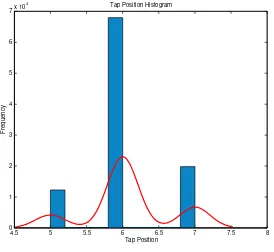
The data indicated that this specific transformer only operates between 3 taps. The categorical labels, which represents these tap positions for the K classes (k = 5, 6, and 7), are encapsulated in the vectorsytrain andytest. The tap values were chronologically mapped to a natural order 1, 2, and 3. Therefore, a ‘1’ is labelled as tap 5, a ‘2’ is labelled as tap 6, and a ‘3’ is labelled as tap 7. The two transformers operate in parallel and have a master-slave configuration. In this case, the tap position data of one transformer is needed to provide the labels1.
The feature matrix consist of the following 19 variables captured from both transformers2:
• Power Factor (T1&T2)
• Reactive Power (T1&T2)
• Apparent Power (T1&T2)
• Frequency (T1&T2)
• Real Power (T1&T2)
• Circulating Current (T1&T2)
• Voltage (T1&T2)
• Power Reserve
• Current (T1&T2)
• Current Phase Degree (T1&T2).
The data was extracted from anOSIsoftR PI server using
a MicrosoftR Excel plug-in. The measurement interval
was set at 30 seconds for a period of approximately 1 month. An interpolation approximation in the PI-Excel
plug-in was used to align asymmetric data measurements. The impact of this on the performance accuracy is dis-cussed in the results section. The 19 normalised features, prior to cleaning, are shown in Figure 1. The data had
0 1 2 3 4 5 6 7 8 9 10
x 104
−25 −20 −15 −10 −5 0 5 10 15 20 25
Examples
Features
Data (Normalised)
Fig. 1. Feauters before data pre-processing.
two empty time zones where nothing was captured and had to be removed. The clean data is shown in Figure 2. A scatter plot was used to view any existing correlations between variables in Figure 4. The diagonal shows the histograms of the variables. The independent assumptions between variables and variable-label correlations were ex-plored in order to select the features. A decision was made to use all 19 variables, since none had significantly high correlations with the labels. An interesting phenomenon was observed between the circulating currents from both transformers shown in Figure 3. The root cause is still being investigated, since the data points are not complying to the y = −x linearity. It is strongly suspected that, it could be the result of the linear estimations provoked
1
Some measurements indicated a very small latency between the master and slave tap transition. This was ignored.
2
T1 andT2represents the two Transformers.
0 1 2 3 4 5 6 7
x 104
−20 −15 −10 −5 0 5 10 15 20
Examples
Features
Data after pre−processing (Normalised)
Fig. 2. Features after data pre-processing.
by interpolation, given that the data measurements are temporarily misaligned.
−100 −80 −60 −40 −20 0 20 40 60
−80 −60 −40 −20 0 20 40 60 80 100
Circulating CurrentT1
Circulating Current
T2
Circulating Currents Scatter plot
Fig. 3. Circulating currents fromT1 andT2.
Fig. 4. Some feature correlations.
0 2 4 6 8 10
Fig. 5. Feature measurements and missing data.
4.5 5 5.5 6 6.5 7 7.5 8
Fig. 6. Tap position histogram.
training. All training and test set data were randomised before training attempts.
2. METHODOLOGIES
In this section, the two models used to predict the tap positions are illustrated. The respective equations for the cost functions and derivatives for each model is shown, along with other key calculations regarding parameter estimations.
2.1 Multi-class Logistic Regression
The logistic classifier h(θi)(x) is trained for each classito predict the probability thaty =i. The one-vs-all method relies on the prediction for each class i, given inputx, by maximising maxi(h(θi)(x)) [1].
In order to classify the three tap positions from the dataset the one-vs-all logistic regression classifier was selected as a baseline performance indicator. The cost functionJ is indicated in Equation 1, with the additional regularisation term3. In order to compute each element in
the summation, hθ(x(i)) needs to be calculated for every
label i, where hθ(x(i)) = g(θTx(i)) and g(z) = 1 1+e−z is
3
Note that the multi-class regression did not train with feature
mapping,L2regularisation was added to penalise possible noise
over-fitting [2].
the logistic function. Note that the bias term should not be regularised.
Correspondingly, the gradient is calculated using the par-tial derivative of the regularised logistic regression cost for
θj. This is shown in Equation 2 and Equation 3 [1].
∂J(θ)
For the dataset, the result of the multiple logistic regres-sion classifier is a matrix θ ∈ RK×(N+1). Each row in
this matrix corresponds to the learned logistic regression parameters for one class.
Am-dimensional vector of labelsywas used for each class
k∈ {1, ...,K}, whereyi∈[0,1] indicates whether thej-th training instance belongs to classk(yj = 1) or a different class (yj = 0).
The multi-class predictions are calculated based on prob-abilities for each class given the input. The output vector with the highest probability is selected as the correspond-ing class label. Results and limitations for this classifier are discussed in the results section.
Introducing nonlinearities to fit more complex decision boundaries comes down to finding a suitable higher order polynomialfeature mappingtransformation. However, this technique can be time consuming and computationally expensive (i.e., O(n2) or O(n3) depending on the order,
wherenis the number of features).
2.2 Neural Network
An easier way to learn more complex nonlinear hypotheses is using a neural network. The neural network in this paper has one hidden layer to introduce the necessary nonlinearities, extracted from the features, to train a more complex decision boundary. This model does not map input features directly to output labels (as in the case of the simpler logistic regression model). Instead, it learns to map input features to an intermediate hidden representation space from which it learns to map to output labels. This results in a more powerful classifier.
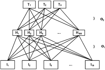
The same dataset was used to train a one-hidden layer neu-ral network shown in Figure 7. The architecture comprises an input layer I, a hidden layer H and an output layer
labels (tap position). As previously explained, the training data is loaded into the feature matrix Xtrain and label vectorytrain. The test set and training set consists of the same data used in the multi-class regression model. The cost function,J(θ) with regularisation restriction,L(θ) is shown in Equation 4 and Equation 5. Training proceeds by minimising the sum, min(J(θ) +L(θ)), by using the
gradi-ent descgradi-ent algorithm. Thesigmoid activation function is
used in this model similar to the one used for the previous model.
Fig. 7. One-hidden layer neural network model.
J(θ) = 1
The gradient is calculated using the standard
back-propagation algorithm for a regularised neural network.
The logistic function is used in this model to introduce the nonlinearities needed to shape the decision boundary. The initial weight value parameter interval forθ(l)is calculated
based on the number of input and output units in the net-work shown in Equation 6. HereLin=slandLout=sl+1
are the number of units in the layers adjacent to θ(l) [1].
Random values between ǫ∈ [−0.52,0.52] was selected to initialise the elements in the two weight matrices. This is a favoured heuristic to break symmetry between connections while training the network. A numerical estimation algo-rithm in [1] was used to perform gradient checking on the forward and back-propagation algorithm before training the network.
The results for this model will be shown in the results section, compared to the results of the logistic regression model. In general, neural networks are powerful, black-box function approximators. They can learn complicated, higher-order dependencies between input variables and output predictions and are well-suited for prediction tasks where these dependencies are unknown.
3. RESULTS
The results for the linear multi-class logistic regression classifier is shown in Figure 8. The training set and test
set accuracy is indicated compared to different values of the regularisation parameter. For no regularisation the training and test set accuracies matches well. The best test set accuracy was obtained with a regularisation constant ofλ= 1. For larger values ofλthe model suffered under-fitting, indicative by divergence between the performance curves.
Accuracy of Train and Test Set
Training Set Test Set
Fig. 8. Multi-class logistic regression model accuracy.
Multi-class logistic regression cannot form complex hy-potheses by itself as it is a linear classifier and only able to find linear decision boundaries. For the dataset used in this exercise it is recommended to create polynomial features from the data, in order to improve the model’s results. Higher-dimensional features will have a more complex de-cision boundary. While feature mapping allows for a more expressive classifier, it is also more prone to over-fitting and depends on regularisation. A regularisation parameter can be selected using a cross-validation set.
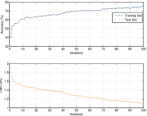
The neural network implementation was able to represent the complexities in the dynamics of the transformer and form nonlinear hypotheses. The performance of the neu-ral network over 100 iterations is depicted in Figure 9. Both the training set and test set accuracies are indicated and correlated well throughout the iterative optimisation process. The cost function monotonically decreased, indi-cating progress towards local or possible global minima. The training set reached a 99.99% accuracy, and the test set a 99.2% accuracy after≈1500 iterations.
Without regularisation, it is possible for a neural network to over-fit a training set so that it obtains close to a 100% accuracy on the training set and much lower accuracies on the test set. This is because the training set is inherently noisy (e.g., due to measurement error). Over-fitting occurs when a powerful model (such as a neural network) starts modelling the noise in the data instead of the true underlying regularities. This causes these models to generalise badly to unseen new test cases (what we ultimately care about).
0 10 20 30 40 50 60 70 80 90 100 30
40 50 60 70 80
Iterations
Accuracy (%)
0 10 20 30 40 50 60 70 80 90 100
1 1.2 1.4 1.6 1.8 2
Iterations
Cost (J(
θ
))
Training Set Test Set
Fig. 9. Neural network model accuracy and cost function.
the entire feature set was used instead. The model seemed to benefit from features representing the inter-transformer dynamics such as the circulating currents and current phase differences.
4. CONCLUSIONS AND RECOMMENDATIONS
In this paper, the development of a statistical model of an on-load tap changer (OLTC) was presented. The goal of this exercise was to validate post-descriptive analytics using recently acquired substation data, and to develop a model capable of predicting the operational OLTC posi-tion. The results indicate the current data to be benefi-cial for this specific task and the model accuracies set a promising foundation in assisting the network operations engineers with the ongoing maintenance of power system integrity. However, for future smart grid system imple-mentations, demanding accurate decision-making ability in complex heterogeneous network environments, higher quality data is imperative.
My biggest concern regarding this exercise was the mis-aligned substation data, due to dissimilar measurement intervals from different relays or delayed data concentrator time-stamping. Although not many of these events were encountered, it is not ideal to train models with such data, with the risk of inaccurate results. In addition, the delta window technique, which is used to track and log larger deviations above or below a certain threshold in the measurements, can contribute to random interval times. This poses a risk to the reliability and use of meta-data. Introducing such randomness is proportional to increasing uncertainty within the model and may provoke confound-ing results. A case in point is Figure 3 in Section 1.1. Here the effect of interpolation on misaligned data points can be seen by inspecting the points not complying to the−x
gradient.
Interpolation reconstructs the intermediate data points within the range of the missing discrete points based on the known (actual measurements) data points. This in itself is a curve fitting or regression approximation (in some cases linear), which can have implications on the model accuracy and increase training time.
It is recommended that an effort is made to alleviate the alignment issues between different relay measurement capturing times and all variable times. It is therefore not recommended to use the delta window practices or compression techniques, specifically for high frequency or impulse measurements. By removing random interval times and synchronising the data, reliable and consistent predictive analytics can be applied using some of the machine learning methods explained in this paper. All relays or devices capturing the measurements should be synchronised as far as possible.
Furthermore, it is recommended that feature extraction analysis and unsupervised learning strategies such as di-mensionality reduction be researched with regard to this specific data set. A performance comparison to a support vector machine methodology is also expected. The data is predominantly low frequency time series data and might not have many degrees of freedom if representing lower order dynamics. In such cases it might be possible to use fewer features in the development of other models, which may reduce training time. Possible on-site data pre-processing can be utilised within the substation and the resulting compressed information communicated back for modelling purposes. This might also alleviate the problem with the communication channel bandwidth constraints.
Future work will include reinforcement learning strategies to accommodate for changing data, and the investigation of Fourier and wavelet transforms as a feature extraction strategy. This will commence supplementary to and in tan-dem with the ongoing Eskom substation data acquisition projects.
ACKNOWLEDGEMENTS
The author would like to extend his sincere appreciation to the following experts for their substantive comments, review, and approval of the paper: Stephan Gouws, Tertius Hyman, Rodney Jose, Ziyaad Gydien, and Erlind Segers.
REFERENCES
[1] Andrew Ng,Machine Learning Class Notes, Stanford Coursera.org, (2012)
[2] David Barber, Bayesian Reasoning and Machine