Provided for non-commercial research and education use.
Not for reproduction, distribution or commercial use.
DEEP-SEA RESEARCH
PART I
H.M.VMAICEM. LS.IIIIODJOHECOIO_ L..,.y;\
l.lfH lhr ch",·pw.ah<r 1nt:>!!,)H IhWLp,h Hit" ィャNャBュ[、ャLiNャイNャBセBセBHLNioo@ }h .. ",lfr,hl.luul\'" iセG@ lo(hlOr".I11111ll>Il\thn\1\!1
yエケNimeエェNmNセ@
Y. uu.D.L\MYJOOWSkI. Ill,' aヲHィゥセLNNiBjZゥャ@lrop""; tn\l,lbohT\ W.lh' mlt'l.lltl"m wuhlnfl'!t' 1.,,1.1['1('"
IA.SOWRU.L XII
000110._
a HIWIS. U I l I S 1 _ 11'itl A \llHI1\1\oIIN'I' NiHャセAyBGセ@ ul I.nulV'" jt.' GijiuャャQBセ|@ ,nl<' QIQLLBGh{セiLioエイNNセャャャャ@ ッNセ@ v,jfI.lbIIJlY''''K'j 1ft \'Nn m th..· ...u!h セイョMAiLュ」@ l\i.lJkh
J. KAJI1.AV.LO£IUUf,A.£Nti.U. 1.:;",1 .\hlUlt1.UU(' .md "'-I!'!!I,mhut"m HII{Jlhp.lrcilt e,np;; セ[tィGQ@
S ェahUャャエエャNqLセjN@ PI(W'JB.. 1>011111.11... nt'" Ill .. ,,,,,.,IIII,.oph..t111 h\;)Unl '" Ih< iャオイセィBェQQ@ N. VAN 00SJ'EJClE. s.. CIlOC*. "",Y (II ヲィセG .1\'
K _ .... LOIOO
G.T, TAYIJlI. lit セ@ I ;>116 iiIG、ャuャセQQQ@ ("t r.:"·llJVnu' LIセ@ \IV!:) .I'''\>' 1.llI",' wnl, GQQセQャHG@ 'tI1«1 .l!}(l
.. VAIIIA. c.1IJrtIITIZ..Ml. I.l1llilOJt HI;G.Inn ;unl'_ !r. WItt 'II "'" .If\t)lllt l ,j(\-#lll A..I\:n
0001 M.l. 5CMHRlIH
jNNセ b. セ⦅@ iャセ@ M.)kxuldf .H'Itd IwtoptC".n,tl.linl' ,}fl Ih(' Wllf< エセ@ nf GLQ|セBサィセゥ@
tセ@ セ@ p.,irl1tOl.111.' O'li!oIOK' (JI/)fin '>11 Ih,' nru:ltwl'\ft'rn
nャNャイjセイnヲjjイエ@
fit. セjNPmPPe。aGB@ ャゥ\セ@ itf'1.1I\()(l'.i'IP 1:lo.'1 ....l"i'nIH''-' セャャャGB@ (Jwun) ョ|jIエイセ@ n QQィセ@ BGョセQ@ セQNャn[G@ ケLセ@ lIIII"'oIZ'Hl."'QU,WHI.I'P.I,dk.lntlllli\fl.l''4.IlI.lIt''!rn'l';!J!:I':h<>i
(1\('\\'r»l('rnl'.«:tlfY"<llmP,",1
( lW'HS. £J. wna Ii 1'1 Mo-!'d'11\' df,,,..H11( ,.u1).-JIl flll)( ..nd GセセQHIゥ」ョ@ PI'I1o<'! セ@.Ir"m I.'f!n I M. 5CtI.011!It. dllTf"\'nr pl.mkton rmWaWI." lOIN: 'o'luth('fl\ Ikl.ln .a.VNI_ICJIFf.
K JDOSQI ....0._
ェNeNセB@ I セLN「@ Ihl' HLエTLLセケ@ .I",d d''!fllmthln "j twmhlf /('l.IrWn!t(,f.l <It 't\{'
A. セ@ ll"kLn i,C<.Hi"1y ,mid セ、ィjBBャ@ "ii'.' 1I.I!,Oh \('.1 la<pe C.W..-rY.P.L£CiINDIII_ I };', hNMNZGセGセiNエャセィャ\@ Irl,)\KJOIl\h1ih ,11!Um.: ""'1' '>\'.1 ィBLuエセiAii\GAヲiGNエ[@ ....',\1 n.Df.SIIlI'VtItEs (.IUll,h.lt tll)':.,;1 '\.0.11.,
www.el•• vier.com/locate/dari
This article Llppenred in a lOUlnul publ:shed Dy ElSe\! . 1 i.l
copy is furnished to the author ior internal non-C0l1lrnerCI,11 I(:search
and education use. including for instruction at the <luttlOfS itLitton
and sl1arinq Wlttl 」ッャャ・Bセャオ・ウN@
Other
llses.
including reproduction and distributllicensing caples. or posting to personal. institutional Dr thild par
websitcs arc proh:bltecL
In most cases authors are permitted to post thou \'(;151011
article (e.g. In Word or Tex form) to エエQHセゥイ@ persona website or institutional repository. Authors reqUiring fUrtner IIllormall
regarding Elseviers archiving and manuscript are
encouraged to VISit:
DeepSea Research I 56 (2009) 12031216
Contents lists available at ScienceDirect
セM
...
--DeepSea Research I
I I SI·\ II
iセ@ journal homepage: www.elsevier.com/locate/dsriThe deepwater motion through the Lifamatola Passage and its
contribution to the Indonesian throughflow
Hendrik M. van Aken
a.*,Irsan S. 8rodjonegoro
b,Indra jaya
c., NIOZ Royal Netherlands Institute for Sea Research. Texel. The Netherlands
" ITB Institute of Technology Bandung, Bandung, Indonesia , IPB Bogor Agricultural University. Indonesia
ARTICLE INFO ABSTRACT
Article histOlY: In order to estimate the contribution of cold Pacific deep water to the Indonesian
Received 28 August 2008 throughflow (ITF) and the flushing of the deep Banda Sea. a current meter mooring Received in revised form has been deployed for nearly 3 years on the sill in the Lifamatola Passage as part of 26 January 2009 the International Nusantara Stratification and Transport (INSTANT) programme. The Accepted 1 February 2009
velocity. temperature. and salinity data. obtained from the mooring. reflect vigorous Available online 7 February 2009
horizontal and vertical motion in the lowest 500 m over the セRPPP@ m deep sill. with
Keywords: speeds regularly surpassing 100 cm/s. The strong residual flow over the sill in the
Indonesian throughflow passage and internal. mainly diurnal. tides contribute to this bottom intensified motion. INSTANT The average volume transport of the deep throughflow from the Maluku Sea to the Lifamatola Passage
Seram Sea below 1250 m is 2.5 Sv (1 Sv = 10" mJ /s). with a transport weighted mean
Current measurements
temperature of 3.2
c.
This result considerably increases existing estimates of the inflow of the ITF into the Indonesian seas by about 25% and lowers the total mean inflow temperature of the ITF to below 13 C. At shallower levels. between 1250 m and the sea surface. the flow is directed towards the Maluku Sea. north of the passage. The typical residual velocities in this layer are low HセS@ cm/s), contributing to an estimated northward flow of 0.91.3 Sv. When more results from the INSTANT programme for the other Indonesian passages become available. a strongly improved estimate of the mass and heat budget of the ITF becomes feasible.c 2009 Elsevier Ltd. All rights reserved.
1. Introduction Gordon (1986) assumed that in the ITF about 8.5 Sv (1 Sv = 106 m3/s) flows in the upper 1000m through
In his description of the warm return flow of the several branches in the Indonesian seas. while diapycnal thermohaline overturning circulation. Gordon (1986) mixing in the ITF maintains a local downward airsea heat stressed that interocean exchange of thermocline waters exchange of about 100W/m2. Simulations with ocean is an essential process to maintain this densitydriven general circulation models as well as with coupled global global circulation system. One of the important exchange climate models have shown that the existence of the ITF processes is the Indonesian throughflow (lTF), which has farreaching consequences for the global ocean transports water from the low latitude Pacific Ocean circulation and climate (e.g. Schneider. 1998; Wajsowicz through the Indonesian seas to the eastern Indian Ocean. and Schneider. 2001; Pandey et al.. 2007).
Hydrographic observations (temperature. salinity. CFCs) have shown that this shallow inflow into the Indonesian seas (full arrows in Fig. 1) occurs mainly through the
• Corresponding author.
Makassar Strait between the islands Kalimantan and
E-mail addresses:[email protected] (H.M. van Aken),
[email protected] (I.S. Brodjonegoro), [email protected] (I. Jaya). Sulawesi (Gordon and Fine. 1996). The shallow Dewakan
09670637/$ see front matter (C. 2009 Elsevier Ltd. All rights reserved.
...
\
I
1204 H.M. van Aken et al. / Deep-Sea Research 156 (2009) 1203-12165
o
-5
10
Indian Ocean
Pacific Ocean
.
•
110 115 120 125 130 135
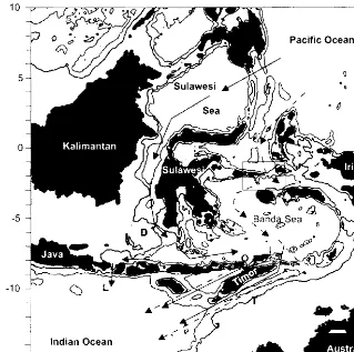
Fig. t. Map of the Indonesian throughflow. The full arrows depict the main shallow throughtlow route via Makassar Strait. The dashed arrows show the deep throughtlow from the Pacific Ocean via the Banda Sea to the Indian Ocean. The full line shows the 2000111 isobath, while the shaded area is shallower than 500111. The area in the rectangle encompasses the llfamatola Passage and is enlarged III Fig. 2. The capitals D, l. 0, and T indicate the approximate locatIOns of, respectively. the Dewakan sill. Lombok Strait. Ombai Strait. and Timor Passage.
sill at the southern end of Makassar Strait (D in Fig. 1) has a sill depth of about 680m (Gordon et al.. 2003b). Current measurements in Makassar Strait have shown that the throughflow through Makassar Strait is about 10 Sv, with a maximum contribution from the layer between 150 and 200m (Gordon et al.. 1999, 2003a). The mean tempe-rature of the throughflow in Makassar Strait is nearly 15 C (Vranes et al.. 2002; Gordon et aI., 2003a). The main exits of the ITF towards the Indian Ocean are the passages between the lesser Sunda Islands (Nusantara), in parti-cular Lombok Strait, Ombai Strait, and Timor Passage (L, 0, and T in Fig. 1, respectively).
Because of the limited depth of the Dewakan sill in Makassar Strait, ventilation of the deep basins in the Banda Sea, with depths in the Weber Deep surpass-ing 7000m, requires another pathway. Van Riel (1956) derived, from the changing temperature stratification measured during the Snellius Expedition in 19291930, that the flushing of the deep Banda Sea follows a pathway from the Pacific Ocean, via the Lifamatola Passage east of Sulawesi (box in Fig. 1, and Fig. 2). The sill in this passage has a depth between 1900 and 2000 m (van Riel, 1956; Broecker et aI., 1986). allowing a deep throughflow with temperatures well below that of the throughflow in Makassar Strait. Van Aken et al. (1988) and Gordon et al. (2003b) have shown, from tracer distributions, that the
hydrographic stratification in the deep Banda Sea agrees with a ventilation by deep overflow from the Pacific Ocean via the Lifamatola Passage. Thereby the cold through-flow water descends from the Lifamatola sill along the topography in an approximately 500 m thick layer, first into the 5000 m deep Seram Sea, and second from the Seram Sea over a 3500 m deep sill into the Banda Sea (Van Aken et al.. 1988). Along this path some heating of the bottom water is observed, mainly attributed to mixing with warmer overlying water near the sills (Van Aken et aI., 1988). Consequent deep upwelling and mixing in the Banda Sea then brings the deep throughflow water from a depth of 5000 to about 1000 m (Van Aken et al.. 1991; Gordon et al.. 2003b). Above the latter level the water from the deep throughflow leaves the Banda Sea towards the Indian Ocean through the southern exits, joining the shallow throughflow water from Makassar Strait over the 680 m deep Dewakan sill.
[image:3.611.99.418.34.351.2]1205 H.M. vall Aken et aI./ Deep-Sea ResearciJ f .56 (2009) 1203-1216
a
(j)
Q)
セ@ 2
ro
...J3
125 126 127 128
Longitue (E)
b
1000
セ@ 1200
E.
1400セ
a. 1600CIl
C
1800 2000
0 5 10 15 20 25 30 35
[image:4.611.91.419.83.468.2]Distance (km)
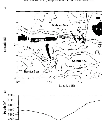
Fig. 2. Plot of the topography near the Lifamatola Passage, between the small Lifamatola Island and the larger Island Obi mayor, with isobaths every
1000 m (a), based on the Smith and Sand well (1997) 2' x 2 resolution ETOPO 2 topographic data set. The cross mdlcates the position of the cllrrent meter mooring near the sill of the passage, while the arrow in the direction 129 shows the observed mean current direction in the lowest 500 m, The line. perpendicular to the vector, ending in dots. is the crosssection for which transports have been calculated, The bottom profile along this line is shown m (b). The mooring was located at x 14.7 km.
30 and 15 cm/s at several depths, Broecker et al. (1986) reported observations with two selfrecording current meters over the sill, each about 10 m above the bottom, which lasted 28 days, They found a typical steady southeastward residual velocity of about 25 cm/s, in agreement with a deep flow of Pacific water towards the Banda Sea. This flow was modified by weaker Hセャo」ュOウI@
diurnal and semidiurnal tides. Van Aken et al. (1988) reported 3.5 months of current measurements with a current meter mooring over the sill. At 60 m above the bottom the mean velocity was 61 cm/s, directed to the southeast, while at 200 m above the sill the mean velocity was 40cm/s, in the same direction, Superimposed on the mean residual flow were tidal motions of a mixed semidiurnal and diurnal character, leading to total velocities in the bottom layer that regularly surpassed 1 mis, From these current measurements the deep inflow below 1500 m was estimated to be 1.5 Sv. Luick and Cresswell (2001) carried out observations with a single current meter mooring, located at 141 'N, nearly 400 km
north of the Lifamatola Passage, in a 2301<01 wide passage of the Maluku Sea east of Sulawesi. Assuming a horizon-tally homogenous flow, they reported a southward transport between 740 and 150001 of 7 Sv, However, one can question whether a Single observational point can be representative for the ocean circulation in that 2301<01 wide passage, especially since the hydrographic observa-tions (T, S, O2 ) indicate the presence of a cyclonic
circulation in the Maluku Sea below 1800 m (Luick and Cresswell, 2001),
H.M. van Aken et al.! Deep-Sea Research 156 (2009) 1203-1216
1206
,
information hampers the validation of ocean general circulation models and global climate models. In response to this lack of knowledge the international Nusantara Stratification and Transport (INSTANT) programme was established to directly and simultaneously measure the ITF. both in the northern inflow passages and in the southern outflow passages (Sprintall et al.. 2004). In this international research programme. scientists from Indo-nesia. the USA. Australia. France, and the Netherlands cooperated to determine the strength of the ITF entering and leaving the Indonesian seas during three consecutive years. Variations in the ITF will be related to changes in the meteorological and oceanographic forcing (sea level. monsoons. EI Nino. Indian Ocean Dipole. etc.). This paper deals with the observations with a current meter mooring over the sill in Lifamatola Passage, carried out during the INSTANT programme. It mainly focuses on the through-flow of the Lifamatola Passage and its variability, but also describes the higher-frequency (tidal) current oscillations in the passage.2. The data
The sill depth in Lifamatola Passage is about 2000 m (Fig. 2). Slightly downstream of the sill a mooring was deployed twice for a period of about 1.5 years. leading to a total mooring period of over 34 months (Table 1). The deployment cruise in january 2004, the service cruise in
Table t
Description of the INSTANT moorings in the Lifal11atola Passage.
july 2005. and the recovery cruise in january 2006 were all carried out with the Indonesian RV Baruna jaya I. During these cruises. series of CTD casts were also recorded, with during each cruise at least one CTD cast close to the mooring position. reaching from the sea surface to the bottom. For the first period the mooring was fitted with two RDI 75 kHz ADeps (Long Ranger). covering the upper and lower parts of the water column. upward looking near the surface. and downward looking in the bottom layer. At intermediate levels, three Aanderaa ReM
11 acoustic current meters were mounted, All RDI and Aanderaa instruments were fitted with a tilt sensor for the correction of the velocity. measured from a tilted mooring. Each of these instruments contained a tempera-ture sensor, while the ADeps were also fitted with a pressure sensor. Additionally five Sea Bird Electronics Microcats (SBE37SM) were mounted to record pressure, temperature. and salinity (Table 1), The mooring position appeared to be about 30 m shallower than the deepest part of the nearby deep channel over the sill, at a distance of about 1 km further northeast. After recovery of this mooring it appeared that because of a faulty but un-documented setting of these instruments, only 7 of the 80 data bins of 8 m length were recorded, strongly diminish-ing the information on the ITF, which is assumed to be concentrated in the near-surface and near-bottom layers. Moreover, it appeared that because of very strong tides the 15-min average velocity at mid-levels regularly surpassed 140 cm/s, This caused a serious blow-down of
Mooring name Latitude Longitude Deployn1ent dale Recovery date Corrected depth (m)
LOCO-1O-1 1 '49.1 'N 12657.S'E 26-01-2004 17-07-2005 2019
Height above bottom (m) Instrument type Serial number Sampling interval (min)
1535 RDI ADCP 3553 30
1534 SBE 37 Microcat 2672 5
1232 Aanderaa RCM 11 243 15
1231 SBE 37 Microcat 2673 5
931 Aanderaa RCM 11 244 15
930 SBE 37 Microcat 2674 5
630 Aanderaa RCM 11 245 15
613 SBE 37 Microcat 2659 5
608 RDI ADCP 3714 30
10 SBE 37 Microcat 2961 No data
Mooring name Latitude Longitude Deployment date Recovery date Corrected depth (m)
LOCO-1O-2 1 49.1'N 12657.S'E 17-07-2005 04-12-2006 2017
Height above bottom (m) Instrument type Serial number Sampling interval (min)
1233 RDl ADCP 3553 30
1231 SHE 37 Microcat 2959 5
931 Aanderaa RCM 11 403 15
930 SHE 37 Microcat 2672 5
630 Aanderaa RCM 11 243 15
613 SSE 37 Microcat 4139 5
60S RDl ADCP 3714 5
1207
H,M. vall Akell er aI./ Deep-Sea Research 156 (2009) 1203-1216
the mooring with an average range of 435 m. adding to the information loss, In the second deployment period the mooring was shortened by 300 m to reduce blowdown, which decreased to an average range of 252 m. However. thereby the possibility to measure velocity in the upper 300 m was lost. The faulty ADCP setting was also repaired, so that effectively in the second period our information on the current structure covered a larger part of the water column. although data reached only to 300 m below the sea surface. The bias in the horizontal velocity. induced by the horizontal motion of the sensors due to the blow-down, was estimated to be about 2
emls
or less, with a periodic character. Since the focus of this paper is on the throughflow, and since the dominant tides have an amplitude of at least an order of magnitude larger. this bias has been ignored.After recovery of the moorings. the recorded directions were corrected for the magnetic variation. and. by a combination of lowpass filtering (filter width セ@ l/h) and subsampling every whole hour. a synchronous hourly data set for all sensors and ADCP bins was produced. including sensor or bin depth. A shift of the time base of each instrument was applied in this process to correct for the effects of different recording intervals and the different meanings of the time stamps in the different instruments (beginning, centre, or end of the recording interval), From these synchronized and depthdependent data, time series of hourly data were calculated at fixed depth levels by means of vertical linear interpolation, every 100 m in the upper 1600 m and every 50 m from 1600 to 2000 m, Continuous hourly data records are available for the interpolation depth interval from 1000 to 1500 m in the first deployment period, and for the 10002000 m depth interval in the second deployment period. In order to recover information on the low-frequency flow in the parts of the water column where data were available only for part of the tidal period because of the mooring blowdown. the monthly mean
residual current was estimated from a harmonic analysis with the dominant tidal frequencies (see below). For the first deployment period this supplied us with monthly mean residual current data from 500 to 1800 m. and for the second period from 300 to 2000 m.
From the average current components between 1500 and 2000 m. measured during the second deployment period, the mean deep current direction was determined to be 129 (arrow in Fig. 2). This direction appears to be well aligned with the deep channel over the sill. In the following discussion we have rotated our geographic reference frame. naming the direction 129 alongchannel. and the direction perpendicular to the channel. 219. crosschannel.
3. The character of the currents and their variability
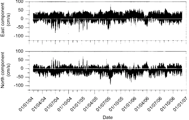
Current data at 1500 m are available for the whole deployment period (Fig, 3). At this level the mean velocity is 14.7
cmls
to the southeast (119 ). The magnitudes of the temporal variation of the current components, expressed as standard deviation. are 20,7 and 17.5cmls
for. respec-tively. the east and north components. The plot of both velocity components (Fig. 3) shows a considerable con-tribution from the tides, with an envelope that shows more or less regular fortnightly variability. indicative of the spring tideneap tide phenomenon, as well as longer-term changes of the residual flow. At 1500 m the tides cause a regular reversal of the current direction. This tidal reversal of the current direction is observed even during spring tide at 2000 m. about 20 m above the bottom, However. during neap tide the residual current at 2000 m is larger than the tidal contribution, maintaining a per-manent southeastward bottom flow. During 0.16% of the 1h data records the current speed at 1500111 exceeds 1 m/s. This fraction increases to 12.6% at 2000 m. Variability at lower frequencies can be observed in the background,100,:,
.,
50 Mセ@
セ@
0·,
1
50 -l
..j
100
i
イBBBtBBBBtMMMtセMMtMMイtセャMMMtMA@
...
TTr'r1100
C
<ll
c:
XNセ@
EJ(? 0
o E
oS
.<:: 50
t::
0
100
z
[image:6.611.126.454.536.745.2]1208 H.M. vall Akell et al. / Deep-Sea Researcll 156 (2009) 1203-1216
leading, for example, to a reversal of the lowpass flow direction at 1500 m during the weeks around 1 April 2006.
The rotary spectrum (not shown) has characteristic tidal bands centred around about N cpd (cycle per day), N being an integer number between 1 and 12. Analysis of the anisotropy of these tidal bands of rotary spectra at the interpolation depths has shown that apart from the semidiurnal tidal bands at 1500 m the variable currents at tidal frequencies are mainly linearly polarized. The characteristic amplitudes of the anticlockwise (ACW) and clockwise (CW) components for those tidal bands were all of the same order of magnitude with ratios ACW/CW varying between 0.7 and 1.4, on average 1.0 (±O.l stdev). As a single exception more extreme values of the ACWICW ratios were found only in the semidiurnal band at 1500 m, where the ACW/CW ratio was 2.7, indicative of the dominance of ACW motion at this depth in this frequency band. This suggests a large influence of the topography on other frequencies and at deeper levels in the channel over the sill. The tidal currents below 1500 m were all aligned in the alongchannel direction.
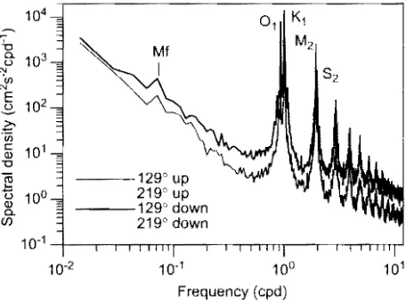
The layeraveraged power spectra for the along-channel and crossalong-channel velocity (Fig. 4) confirm the conclusion, presented by Van Aken et al. (1988), that the tidal current in the Lifamatola Passage is dominated by the diurnal (0) and Kd and semidiurnal (M2 and 52) frequencies, while additional peaks are found at their higher harmonics, at セn cpd (N 3,4,5, ... ). Additionally, a spectral peak is found near the lunar fortnightly (Mf) frequency (7.32 x 1O2 cpd). The latter is close to, but not coincident with. the local inertial frequency of 6.37 x 10 2
cpd. The difference of the spectra for the alongchannel and crosschannel components shows that in the depth interval from 1600 to 2000 m. completely surrounded by the channel wall (thick lines in Fig. 4), the kinetic energy
104
b
0.
103
L) N
'<1) N
E
,£. 102
C
'iii
c:
(l) 101
"0
セ@
L)(l) 10°
0. (j)
10-1
10-2 10'1 100
---129° up
2190 up
---129° down
219c'down
[image:7.611.25.253.522.691.2]Frequency (cpd)
Fig. 4. Power spectrum of the velocity components in alongchannel (129. black lines) and crosschannel (219, grey lines) direction, averaged over the depth intervals 10001500m (up. thin lines) and 16002000m (down, thick). The peaks at the dominant semidiurnal and diurnal tidal component as well as the lunar fortnightly components are identified. These spectra are based on successive 70day subperiods during the second deployment penod, with an overlap of 35 days.
of the alongchannel velocity variations is on average 19 times the kinetic energy of the crosschannel variations at diurnal and semidiurnal frequencies. At the subdiurnal frequencies below 0.5 cpd that ratio for the spectral continuum is about 3, at supersemidiurnal frequencies about 2.3. This anisotropy reflects the fact that over the sill the variable motion takes place in a narrow channel, 8.5 km wide at the depth of the 1800 m isobath. which hinders the crosschannel motion considerably. At the level from 1000 to 1500 m the channel is much wider (28 km at the 1250 m level). and consequently the anisotropy of the variable motion is smaller, セU@ at the tidal peaks, セR@ at subdiurnal frequencies. and セ 1.2 at supersemidiurnal frequencies.
To show the character of the tides in more detail, a harmonic tidal analysis of the data has been carried out for the fortnightly, diurnal, and semidiurnal tides, in-dicated in Fig. 4. as well as for higher harmonics. up to at least セLV@ cpd tides. It appears that the strongest tides are. in order of amplitude. K], 0), M2• 52, and Mf, all five with
amplitudes at all depths between 1000 and 2000 m of over 1
cm/s
in the alongchannel direction. The determi-nation coefficient (correlation R squared) of the harmonic analysis shows that these five tidal frequencies determine on average 65% of the alongchannel current variation1209 H,M. van Aken et aI./ Deep-Sea Researcli I 56 (2009) 1203-1216
30 30
20 20
!!? E
10 C
セ@ 10
(l)
o
§ 0
a.
E
10
8
10 enN 20 20
30 30
1/
30 Mf
20
10
o
10
20
30
30
c;; 20
E
2 10
C
(l)
§ 0
a.
E
8
10en
N 20 30
30
20
10
o
-10
-20
30
-20 -10 0 10 20 -20 -10 0 10 20 -20 -10 0 10 20
219'" component (cm/s)
- - - - 2000m
- - - - - 1800 m
1500 m 1000 m
-20 -10 0 10 20 -20 -10 0 10 20
2190
component (cm/s) 2190
[image:8.611.90.450.101.451.2]component (cm/s)
Fig. 5. Plots of the tidal ellipses at depths of 2000, 1800. 1500. and 1000111 for the tidal components 0,. K,. M,. Sb and Mf. These ellipses were determined with a harmonic analysis of the 、・ーエィセゥョエ・イーッャ。エ・、@ current data from the second deployment period.
4. The mean current profile
For the first deployment period uninterrupted inter-polated hourly velocity data are available for the depth interval of 1000-1500 m, for the second deployment period from 1000 to 2000 m. Only for these depth intervals can the residual currents be determined directly by averaging of the hourly data. To extend the information on the residual currents further in the vertical, we have applied an alternative method. As shown above. most of the current variability comes from only five tidal compo-nents plus sub-tidal variability with time scales from months to years. Assuming that the along-channel current can be described quite well as a monthly mean residual current plus tidal contributions from the OJ, K1• M2 , 52,
and Mf components, harmonic analysis by means of mUltiple linear regression (Emery and Thomson, 1997) can be used to estimate the monthly mean along-channel current components. This can also be applied to those parts of the water column where, because of the blow-down of the moorings, the current record is not contin-uous. but interrupted by short periods of missing data. This has allowed us to extend the mean current profiles. based on monthly averages of the residual velocity. for the first deployment period to the depth interval from 500 to
1700 m. and for the second deployment period from 300 to 2000m.
The current profiles for the two different deployment periods. derived from the monthly mean residual currents (grey lines in Fig. 6). are quite similar to each other. The resulting long-term averaged current profile (black line with symbols in Fig. 6) shows a strong southeastward overnow in the lowest 750 m over the sill. following the axis of the channel. From 300 to 1200 m a small but significant northwestward now of about 3.2 (±0.5 stderr)
cmjs is observed. In the deep overnow the average along-channel velocity reaches a maximum of 67 (-I-6 stderr)
cmjs at 1950 m. about 70 m above the bottom. decreasing downwards to 51 cmjs at 2000 m.
1210 HM. van Aken et al. / Deep-Sea Research I 56 (2009) 1203-1216
250
500
J
750
E
1000.r:
a.
0
<1)
1250
1500
1750
o
20 40 60 801290
[image:9.611.24.250.99.322.2]Velocity Component (cm/s)
Fig. 6. Mean profile of the alongchannel current component (129. black line with symbols) and estimated accuracy (twice the standard error). derived from monthly mean values. with separate curves (grey lines) for the first and second deployment periods. The crosses show mean velocities from the literature. shifted vertically to the appropriate distance from the bottom (L = Lek, 1938; B Broecker et al.. 1986; vA Van Aken et aI., 1988).
profile level at 2000 m was about 20 m above the bottom. The information available from our current profile shows that the southeastward deep overflow extends from the bottom to a depth of about 1250 m, while Van Aken et al. (1988), with data from only two current meters. derived from extrapolation a current reversal at 1500 m. Their averaged velocities were also smaller than those pre-sented here. Therefore it can be expected that the average transport in the deep overflow presented here is larger than their estimate of 1.5Sv.
5. The temperature and salinity stratification
The depth over which the temperature sensors in the mooring moved, because of the blowdown of the mooring, was in general of the same order of magnitude or larger than the expected vertical tidal migration of the isotherms of a few 100m (Van Aken et aI., 1988). Therefore, enough observations were available in the water column between 500 and 2000 m to determine the longterm HセS@ years) mean profiles of potential temperature and salinity (Fig. 7). These show a salinity minimum at セXPP@ m. where in the South Pacific Ocean a similar minimum is found (Wyrtki. 1961). In the lowest 400 m, where the core of the overflow of deep Pacific water into the Seram Sea/Banda Sea system is expected (Van Aken et aI., 1988) the vertical gradient of salinity and potential temperature is larger than directly above this layer.
While during the first deployment period the near- bottom Microcat was defective, during the second deploy-ment period this instrubottom Microcat was defective, during the second deploy-ment recorded continuously the
Salinily
346 34.61 34.62 34.63
I
UPPセMMMMセMMセMMセセセMMセMMMMGWMセ@
s
1000
1500
2 4 6 8
Potential Temperature (CC)
Fig. 7. Mean profiles of potential temperature (thick line) and salinity (thin line) between 500 and 2000111. averaged over the whole deployment period.
nearbottom temperature and salinity in the lowest 10 m. Similar to the velocity signal, the temperature and salinity signals show a strong tidal variability (Fig. 8), with a clear fortnightly variatIOn in amplitude. The temperature and salinity variations are negatively correlated as can be expected from the mean stratification with oppOsite
e
and 5 gradients, depicted in Fig. 7. Therefore the tidal signals of these parameters are in opposite phase. with temperature maxima coinciding with salinity minima (Fig. 8). The spectra of temperature and salinity, derived from this time series (Fig. 9), clearly show the presence of the same dominant tides, which are also observed in the velocity spectrum, including the higher harmonics of the tides. The tidal character of these scalars is therefore also mixed diurnal and semidiurnal. [image:9.611.278.510.100.355.2]1211
H.M. van Aken et al. / Deep-Sea Research I 56 (2009) 1203-1216
3.2 セMMMMMMMMMMMMMMMMMMMMMMMMMMMMMMMMMMMMMMMMMMMNMセTNVT@
Q'
3.0:::l 2.B
J
10 セ@
\-GJ
,
J
a.2.6 E
セ@ 2.4
セ@
C
GJ 2.2
15
a.
2.0 S
",.' 1'1 , 34.62
1-Apr-06 1-May-06 1-Jun-06 1-Jul-06
[image:10.611.100.423.86.236.2]Date/Time (UTC)
Fig. 8. Continuous plot of the nearbottom temperature (black line) and salimty (grey hne). measured wIth an SBE MlCrocat for the sulJpenod April untIl June 2006.
10-'
Mf 10-2
Nセ@ 10.3 Ei spectrum
<f) t::
GJ
'tl
10-4 1§
U S spectrum
GJ 10.5
a. (f)
106
10.7
10.2 10" 10° 10'
[image:10.611.275.507.279.518.2]Frequency (cpd)
Fig. 9. Power spectra of the nearbottom temperature (black line) and salimty (grey line). measured with an SBE Minoeat III the second deployment penod.
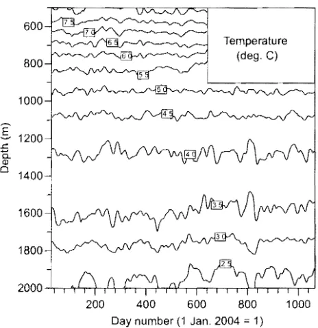
has even a negative extreme of 0.27. The Significant positive correlation is due to the apparent simultaneous upward or downward movements of thick layers of water with their isotherms, reflected by coincident upward or downward peaks in the isotherms (Fig. to). However. at larger vertical distances of about 500 m the correlation is reduced to near zero by additional intrusions of thick packets of water with variable vertical temperature gradients. while the temperature near the bottom is partly in counterphase with the temperature at 1300 m. as can be expected when thermostads are a dominant feature in the variable temperature structure. The stron-gest example of such a low T gradient intrusion occurs between days 800 and 840 (10 March-19 April 2006). In that sub-period the 2.5 and 3.0 C isotherms move down-wards. while the 3.5 and 4.0 C isotherms move up-wards, all over a vertical distance of over 100 m (Fig. to).
Apparently a deep thermostad with a low vertical stability. centred around 1700 m. passed Lifamatola Passage around day 822 (1 April 2006). Such a thick thermostad may have dynamic consequences for the deep flow, since it is probably also connected with changing horizontal density gradients. Evidence for this hypothesis can be seen in the
600
BOO
1000
E
1200.c.
c..
GJo 1400
1600
1BOO
Temperature (deg. C)
200 400 600
BOO
1000Day number (1 Jan. 2004
=
1)Fig. 10. Tlllle-depth sectIon of the temperature measured with the temperature sensors on the moorIng. The sign.!1 was smoothed with a low-pass filter with a width of 14 days to remove the tidal contributions to the temporal variability,
velocity already at 1500 (Fig. 3), which shows a current reversal around that same date.
[image:10.611.17.248.283.450.2]1212 H.M. van Aken et al.! Deep-Sea Research I 56 (2009] 1203-1216
show that the thermostad was much longer than the width of the channel. This suggests that the thermostad was advected from the Maluku Sea to the Lifamatola sill. The cause of the formation of such deep thermostads
J
upstream of the passage remains uncertain yet. The (relatively large size of the thermostad in the alongflow direction ensures that the change of the pressure gradient due to the presence of a thermostad probably extends over the whole Lifamatola sill, and thereby influences the whole deep overflow.
6. Transports through Lifamatola Passage
With the velocity data, obtained from the moorings, we can calculate the volume transport across a section that runs perpendicular to the mean alongchannel deep flow in the direction of 219 . The endpoints of that section are given in Table 2. The section runs from a ridge, extending northwestwards from Obi mayor (depth 1090 m) across the deep channel in the Lifamatola Passage (maximum depth セRPUP@ m) to a "shallow" platform eastsoutheast of Lifamatola (depth 1645 m). The width of this section is 36.2 km, while at 1750 m it is only 10.5 km wide, intersected by the bottom topography (Fig. 2b). For the calculation of the transport we assume that the measured velocity profile (Fig. 6) is representative for the vertical velocity structure across the whole section. For the levels below the deepest interpolated velocity level, 2000 m, we apply the 2000m velocity. Given the narrow width of the deep channel at these levels, the effect of this, or any other extrapolation, is very small.
[image:11.611.30.434.511.735.2]The alongchannel volume transport Tf over the sill between the depth levels Zo and ZI has been computed
Table 2
EndpOInts of the transport section, through which the transports ,lre calculated.
latitude Longitude
139.90'$ 127 05.14'E
1 55.07'5 12652.81'E
from the profile of the velocity in the direction of 129 by the following integral:
Tf =
l,11
VI29 W(z)dz. (1)where W(zl is the depthvarying width of the channel. We have calculated the volume transports for the depth intervals 4501250m and from 1250 to the bottom, since the alongchannel velocity profile in Fig. 6 suggests that in these depth intervals the current is, respectively, in the northwestern and southeastern direction. These depth intervals are well covered by velocity estimates for the second deployment period, but for the first deployment period, part of the data in these intervals are missing in all or part of the months in this period. In order to prevent a possible bias in the transport estimate due to missing data, we have to find a method to obtain a reliable approximation for the transport for the first deployment. For the second deployment period, with a complete data coverage for both depth intervals, the deep transport below 1250 m has been derived from the 5day running mean values of the interpolated alongchannel velocity. The resulting transport time series varies from 0.8 to 5.2 Sv, with an average value of 2.7 Sv ( 1.3 Sv stdev). This transport is nearly twice the transport value of 1.5 Sv derived by Van Aken et al. (1988). This is partly because their 3.5 months of observations gave lower velocity values (vA crosses in Fig. 6) than our 1.5year deployment period, and partly because their estimate of the thickness of the overflow layer (460 m
1
from linear extrapolation was smaller. The best linear correlation between the volume transport and the velocity at a single level(R 0.993) is found a t a depth of 1500 m. The time series at this level is also complete for the first deployment period. We have calculated the volume transport for this period from the velocity at 1500 m by means of tile linear regression with the alongchannel velocity at 1500 m, derived from the data in the second deployment period.
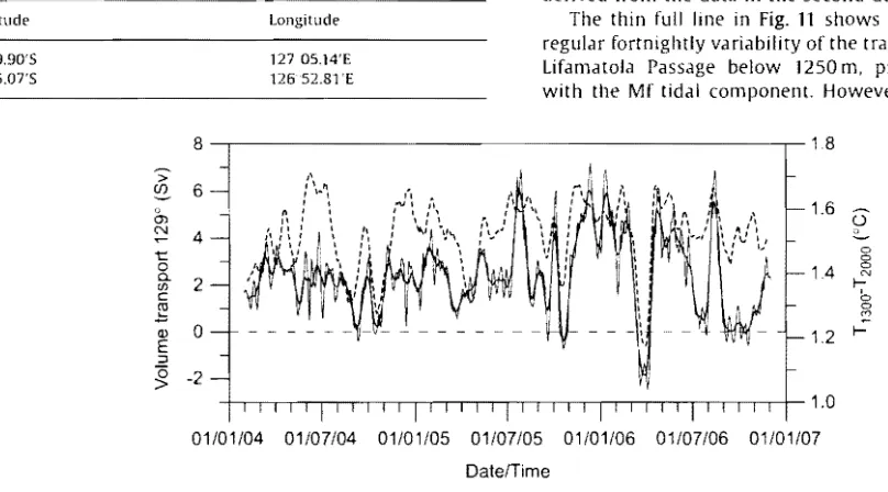
The thin full line in Fig. 11 shows that there exists a regular fortnightly variability of the transport through the Lifamatola Passage below 1250 m, probably connected with the Mf tidal component. However. application of a
1.6 8 , . . 1 8
6
0
4 Q
0
t 0
o 1.4 N0
a.
l-rf) 2
i:, c
0
セ@ I-
""
Q) 0 1.2
E
::::>
セ@ -2
hrr"rr;,.,..r,",,rr.,.,..r,,,,,rr.,.,..r!1 . 0
01/01/04 01/07/04 01/01/05 01/07/05 01/01/06 01/07/06 01/01/07
DatefTime
1213
H.M van Aken et al. / Deep·Sea ResearciJ 156 (2009) 1203-1216
15day running mean (thick full line in Fig. 11) effectively suppresses this tidal contribution. A peculiar phenomen-on in the transport time series is the 22-day period around 1 April 2006. where the along-channel volume transport below 1250 m is negative. It appears that this is caused by the lowering of the zero-velocity interface. on average at -"1250 m. to a level of nearly 1700 m. the deepest current reversal level observed in our records. This lowering coincides with the presence of the thermos tad in the passage. centred around the same depth of 1700 m. as described above. A similar phenomenon. although less extreme. occurred around 20 October 2005. Apparently the vertical temperature gradient is related to the strength of the deep throughflow. The temperature difference between 1300 and 2000 m. assumed to be representative for the vertical temperature gradient in the deep through-flow and the presence of thermostads (Fig. 11. dashed line). shows a regular coincidence of high- or low-transport events with high or low temperature gradients,
The along-channel transport. derived from the IS-day running mean time series in Fig. 11. averaged over the whole near-3-year deployment period. amounts to 2.4
(± 1.5 stdev) Sv. while the transport derived from the averaged profiles in Fig. 6 amounts to 2.5 Sv. Apparently the averaged velocity profile is not very sensitive to the bias caused by levels with incomplete data from the first deployment period.
In order to determine the average temperature of the deep throughflow below 1250 m. we have to determine the weighted mean temperature. The transport-weighted temperature T[W is defined as
(2 )
Trw
where
Hz)
is the depth-dependent temperature. observed with the temperatures sensors in the mooring and Tr is defined in (1). When we calculate the long-term mean value of this T[W with the 5-day-averaged time series of the along-channel velocity and temperature for the second deployment period. we obtain a mean transport-weighted temperature of 3.21 C. while the use of mean vertical profiles of temperature and velocity for this period results in a mean temperature of 3.25 C. Appar-ently the effects of any Reynolds terms in the total heat (temperature) transport are negative. but small. and can be ignored. For the total 34-month deployment period the mean temperature of the deep throughflow. derived from the long-term mean profiles of temperature and along-channel velocity. is 3.22 C. The mean salinity of the deep throughflow. determined similarly. is 34.617. agreeing with the (near-homogeneous) salinity in the deep Banda Sea below 2000m (34.615-34.620; Van Aken et a!.. 1988. 1991l.
In the layer from 250 to 1250 m a significant mean velocity from the Maluku Sea to the Seram Sea is observed (Fig. 6). Given the increasing width of the Lifamatola Passage from 1250 to the sea surface. the assumption that the transport at these levels can be estimated from velocity measurements at a single mooring becomes questionable. But if we do this. the total volume transport in the 1000 m thick layer between 250 and 1250 m
amounts to -1.0 (= 1.1 stdev) Sv. which means a strongly varying. but on average northwestward. transport towards the Maluku Sea. An annual cycle of the northwestward velocity can be discerned only at 300 and 400m depth. in counter-phase with the near-surface Ekman Transport at 7 S in the Banda Sea (Sprintall and Liu. 2005). If we assume that the residual velocity at 300 m extends to the sea surface. we arrive at a small residual northwestward transport in the upper 1250 m of 1.3 Sv. However. estimates of the current structure in Makassar Strait have shown that the vertical current structure in the upper 300 m of the Indonesian seas may show a considerable seasonal variability (Gordon et al.. 2003a). These esti-mates of the transport above 1250 m, given above, are probably not very accurate, and should be interpreted with care.
7. Discussion
The data obtained with the INSTANT mooring in the Lifamatola Passage show that vigorous motion occurs in the deep channel across the sill. That motion consists of the residual flow. contributing to the deep ITF of cold water from the Pacific Ocean towards the Banda Sea and of vertically varying internal tides. Since the southern exits of the Banda Sea are all shallower than the sill in the Lifamatola Passage. this sill controls the deep throughflow from the Pacific to the Indian Ocean (Gordon et al.. 2003b).
In the tidal motion the diurnal tides KI and 0 1 are dominant. although Wyrtki (1961) has reported that in the sea areas around Sulawesi. also in the Lifamatola Passage, the surface tide is mixed, but prevailing semi-diurnal. Apparently the mooring was not intersected directly by a semidiurnal internal tidal wave beam. Generation of (lower-frequency) diurnal internal tides by interaction of the barotropic tide and topography in a stratified sea requires a smaller critical bottom slope than the generation of the (higher-frequency) semidiurnal internal tides. while a propagating diurnal internal wave beam will also follow a less-steep path than the semidiurnal tide (Gill, 1982). The steeper critical bottom slope is probably found deeper on the sill. at a larger distance from the mooring near the top of the sill, than the smaller slope, where diurnal internal tides are generated. The shorter distance to the critical slope combined with the less-steep wave beams will favour the diurnal tide to reach the mooring. These frequency-dependent differ-ences in generation areas and wave propagation may explain the observed local dominance of the diurnal internal tides over the sill.
1214 H.M. vall Aken et oJ.; d・・ーセs・。@ Researcll J 56 (2009) 1203-1216
value. This value agrees with the large vertical motion of the isotherms presented for periods of 4 days by Van Aken et al. (1988). who show depth variations of isothermals (peaktrough) of about 400 m (their Fig. 8). This result also indicates that it is hard to derive the near-bottom vertical stratification from only a few CTD casts. More detailed modelling studies on the generation of internal tides. in combination with resulting generation of turbulent mixing in a general circulation model. like those carried out by Koch-Larrouy et al. (2007). may shed light on the question where and how internal tides contribute to the enhanced turbulent mixing in the deep Indonesian seas. derived by Van Aken et al. (1988,1991 ).
The main transport in the Lifamatola Passage. respon-sible for the cold part of the ITF and the ventilation of the deep Banda Sea. appears to be concentrated in the lower layer of the water column below 1250m (Fig. 6). with a velocity maximum of over 65
cmls
at セ 70 m above the bottom. The observed downward decrease of the velocity below that level is probably related to friction effects in the near-bottom layers. The long-term mean volume transport in this cold ITF, estimated in different ways. amounts to 2.4-2.5 Sv for the total 34-month deployment period. This is nearly 60% higher than the volume transport of 1.5 Sv. derived from a much shorter deploy-ment period of only 3.5 months. reported by Van Aken et al. (1988). This difference is not necessarily connected with long-term changes. From our 34-montl1 transport record (Fig. 11) one can derive that on average 15% of the 3-month-average transports have a magnitude of 1.5 Sv or less. It can be concluded that the relatively low transport, reported by Van Aken et al. (1988), is not really a rare event.The time series of the cold transport, shown in Fig. 11, shows an occasionally strong variation with a time scale of about 1 month. It has been shown that the negative-transport event around 1 April 2006 coincided with the presence of a deep hydrographic feature centred at 1700 m, characterized by a strongly reduced vertical temperature gradient. a thermostad. Below 1700 m the residual flow was then still directed towards the Seram Sea, with near-bottom velocities at 1950 m of well over
40
cm/s.
The negative correlation between the tempera-ture at 1950 and 1300 m suggests that variations in the vertical temperature gradient. as they occur in a thermo-stad, are a dominant feature below 1250 m. To analyze whether the relation between the presence of a thermo-stad in the lowest 750 m and the reduction of the deep overflow can be generalized. we have determined the correlation between the 15-day running mean of the volume transport below 1250 m and the temperature difference between 1300 and 2000 m. The resulting correlation is 0.62. Apparently. deep thermostads are encountered regularly in the Lifamatola Passage. and they cause a decrease in the volume transport. The source and dynamics of these deep features are unknown yet, but the coincidence of the strong thermostad at 1700 m with the low-transport event, as well as the significant correlation between transport and vertical temperature gradient, suggests that both are related.The long-term averaged deep transport derived from our data. 2.5 Sv, is considerably smaller than the south-ward transport between 740 and 1500 m of セ 7 Sv. derived by Luick and Cresswell (2001) for a section in the Maluku Sea between Sulawesi and Halmahera. The transport over a similar depth interval derived from our mooring data, is -0.3 Sv, directed to the northwest. This large contrast clearly indicates. as was already suggested by Luick and Cresswell (2001), that the assumption that the averaged current data from a mooring at the extreme western side of a 230 km wide section are representative for the entire width of this passage is indeed doubtfuL Representative deep current observations are more likely obtained for our section of only 36 km wide. although even in this case the lateral homogeneity is still an assumption. not yet a proven fact. At shallower levels of. e.g .. 500 m the cross-channel distance between the isobaths in the Lifamatola Passage is about one third of the section used by Luick and Cresswell (2001), but even over such a distance it is doubtful that the use of a single current meter moor-ing will produce an accurate estimate of the shallow transport.
The inflow of cold water through the Lifamatola Passage, in addition to the main ITF branch through the Makassar Strait, influences not only the volume budget of the ITF but also the heat transport. The existing transport estimate of the strength of the warm Makassar Strait branch based on the Arlindo Experiment (Gordon et al.. 1999) is 9.3 Sv. The deep inflow through Lifamatola Passage, presented here, adds over 25% of cold water to this estimate. Vranes et al. (2002) derived the transport-weighted temperature in Makassar Strait by four different methods and found a mean value of 14.6 (± 1.8 stdev) C. If we combine these (non-contemporary!) results with the mean transport and transport-weighted temperature from the deep transport in Lifamatola Passage (2.5 Sv and
3.2 C). we arrive at a total northern inflow of the ITF into the Indonesian seas of 11.8 Sv, with a transport-weighted mean temperature of about 12.2 C. This temperature is considerably lower than the temperature estimates from the past of well over 20 C (Gordon et aI., 2003). When considering these results, one has to be aware that these results are obtained by putting together data collected from different experiments, carried out over different years. But new data from all the different contemporary experiments of the INSTANT programme may lead to a thorough revision of the heat budget of the ITF.
1215
H.M. van Aken et al. / Deep-Sea Researcl1l 56 (2009) 1203-1216
suggest a deep maximum in this throughflow at セ 1000 m depth (Sprintall et aI., 2009). At that level the Banda Sea has a mean temperature of セUNP@ C (Van Aken et aI., 1988). The heat transported by 2.5 Sv at 5 C is larger that by the same volume transport in the Lifamatola Passage at 3.2 C.
This implies that the heat flux of the deep throughflow in the Band Sea is divergent, and extra heat has to be supplied to warm the upwelling cold water (Munk, 1966; Van Aken et aI., 1991). This heat source is supplied by turbulent mixing with the overlying water. Given that the
2
surface of the Banda Sea is セVNW@ x 1011 m , and the specific heat of sea water is about 4000 j/kg/ C. the downward turbulent heat flux in the Banda Sea at a level of 1000 m should supply 28 W/km2 to support the divergent advec-tive heat flux. If the cold throughflow rises up to the shallower level of 500 m, where the mean temperature is 8 C (Van Aken et aI., 1988), a downward turbulent heat flux of 74 W/m2 is required. Upwelling of the cold ITF to even shallower and warmer levels needs even larger heat inputs. This heat is supplied by the cooling of the overlying water, and ultimately by cooling of the atmo-sphere in Indonesia. Apparently, maintenance of the deep throughflow through the Lifamatola Passage may have a considerable influence on the local climate, of the same order of magnitude as the heat flux sustained by the throughflow of thermocline water HセQPP@ W /m2) proposed by Gordon (1986).
The downward turbulent heat flux in the water column is balanced by the upward advective heat flux. Using the vertical advection-diffusion model, proposed by Munk (1966), and using a deep transport estimate of 1 Sv, Van Aken et al. (1988,1991) were able the estimate the turbulent diffusion coefficient in the Banda Sea to be 9 x 10⁻⁴
m 2/s. Given a known temperature stratification in the Banda Sea, the turbulent diffusion coefficient derived from Munk's model is proportional to the vertical upwelling velocity, which is in its turn proportional to the deep inflow of cold water. With our new estimate of an inflow of 2.5 Sv, this leads to an estimate of about 2.2 x 10⁻³ m 2/s, more than a factor of 20 higher than
the generally accepted canonical value of 10-4 m 2/s for the world ocean (Gargett, 1984). Apparently, the strong internal tides in the Banda Sea contribute strongly to the turbulent energy budget responsible for the maintenance of the downward turbulent heat flux and the considerable mixing in the Banda Sea (Van Aken et aI., 1988; Koch-Larrouy et aI., 2007).
When more results from the INSTANT programme become available, it is likely that a more reliable budget for the ITF of mass, heat, and freshwater than currently available can be produced. These will form a benchmark for model simulations of the interocean exchange be-tween the Pacific and Indian Oceans and are expected to boost our understanding of these processes for the oceanic climate.
Acknowledgements
We thank the captains and crew of the Baruna jaya I of the Indonesian Agency for Research and Application of
Technology (BPPT) and the technicians and scientists from the Agency for Marine and Fisheries Research (BRKP) for their support during the research cruises. Many Indone-sian students also participated in the three cruises. Theo Hillebrand and Sven Ober prepared and serviced the instruments, while Marcel Bakker, jack Schilling, and Leon Wuijs were responsible for the construction and handling of the mooring, and Kees Veth replaced HMvA during the last cruise. Funding for the mooring equipment was received from the Netherlands Foundation for Scientific Research (NWO) via the LOCO investment programme, and via the IMAU of Utrecht University from the COACh International Research School. Ship time of the RV Baruna jaya I was made available by the BRKP.
References
Broecker, W.S., Patzert, W.e., Toggweiler, JR., Stlllver, M., 1986. Hydro-graphy, chemistry, and radiOisotopes In the southeast ASian waters. journal of Geophysical Research 91, 14,345-14,354.
Emery, W.J., Thomson, R.E., 1997. Data Analysis Methods In Physical Oceanography. Pergamon, Oxford, p. 634.
Ffield, A., Robertson, R., 2005. Indonesian seas finestructure vanabliity. Oceanography 18, 108-111.
Gargett, A.E., 1984. Vertical eddy dlffuslvlty 111 the ocean II1tenor. Dynamics of Atmospheres and Oceans 42, 359- 393.
Gill, A.E., 1982. Atmosphere-Ocean DynamICS. AcademIC Press, London, p.662.
Gordon, A.L., 1986. Interocean exch<lI1ge of thermocline water. journ<ll of GeophYSical Research 91, 5037-5046.
Gordon, A.L., Fine, R.A., 1996. Pathways of water between the Pacific and Indian oceans 111 the IndoneSian sea. Nature 379, 146-149. Gordon, A.L., Susanto, R.D., Ffield, A., 1999. Throughflow within Makassar
Strait. Geophysical Research Letters 26, 3325-3328.
Gordon, A.L., Susanto, R.D., Vranes, K., 2003a. Cool Indonesian through-flow as a consequence of restricted surface layer Ilow. Nature 425, 824-828.
Gordon, A.L., GiullVi, e.F., lIahude, A.G., 2003b. Deep topographic barriers within the Indonesian Seas. Deep-Sea Research II 50, 2205-2228. Koch-Larrouy, A., Madec, G., Bouruet-Aubertot, 1'., Gerkema, T., Bessieres,
L., Moicard, R., 2007. On the transformation of Pacific water Into Indonesian throughflow water by II1ternal tidal nllxlng. GeophYSical Research Letters 34, L04604.
Lek, L., 1938. The Snellius Expedition in the eastern part of the East Indian Archipelago 1929-1930. Vol. II: Oceanographic results. Part 3: Die Ergebnisse del' Strom- und Seriemessungen (in German). Luick, J.L., Cresswell, G.R., 2001. Current measurements In the Maluku
Sea. journal of Geophysical Research 106, 13953-13958.
Moicard, R., Fieux, M., Swallow, j.e., lIahude, A.G., BanJarnahor, J., 1994. Low frequency variability of the currents in Indonesian channels (Savu-Rotl and Rotl-Ashmore Reef). Deep-Sea Research I 41, 1643-1661.
Moicard, R., Fleux, M., lIahude, A.G., 1996. The Indo-Pacific throughflow in the TlI1lOr Passage. journal of GeophYSICal Research 101. 12,411-12,420.
Molcard, R., Fieux, M., Syamsudll1, F., 2001. The throughflow within Ombai Strait. Deep-Sea Research I 48,1237-1253.
Munk, W.H., 1966. Abyssal reCIpes. Deep-Sea Research 13,707-730. Murray, 5.1'., Arief, D., 1988. Throughflow IIlto the Indian Ocean through
the Lombok Strait, january 1985-january 1986. Nature 333,444-447. Pandey, V.K., Bhatt, V., Pandey, A.e., Das, I.M.L., 2007. Impact of IndoneSian throughflow blockage on the Southern Indian Ocean. Current Science 93, 399-406.
Schneider, N., 1998. The Indonesian throughflow and the global climate system. journal of Climate II, 676-689.
Smith, W.H.F., Sandwell, D.T., 1997. Global sea floor topography from satellite altimetry and ship depth soundings. Science 277, 1956-1962.
1216 HM. van AkeTl et 01. / Deep-Sea Researcirl 56 (2009) 1203-1216
Sprintall. J.. WiJffels. S.E.. Molcard. R .. Jaya, I., 2009. Direct estimates of the Indonesian Throughflow entering the Indian Ocean: 20042006. Journal of Geophysical Research, in press.
Sprintali, J., Lill, W.T.. 2005. Ekman mass and heat transport in the Indonesian seas. Oceanography 18 (4). 8897.
Tomczak. M., Godfrey, ].5 .. 1994. Regional Oceanography. and Introduc-tion. Pergamon. Oxford. p. 422.
Van Aken, H.M .. PunJanan. J .. Sairnima, S .. 1988. Physical aspects of the flushing of the East Indonesian basins. Netherlands Journal of Sea Research 22,315-339.
Van Aken, H.M .. van Bennekom, A.J.. Mook. W., Postma. H., 1991. Application of Munk's abyssal recipes to tracer distributions in the deep waters of the South Banda Sea. Oceanologica Acta 14,151-162.
Van Riel. P.M.. 1956. The Snellius Expedition in the eastern part of the East Indian Archipelago 1929-1930. Vol. II: Oceanographic results. Part 5: The bottom water. Ch. II: Temperature.
Vranes. K.. Gordon, A.L.. Ffield. A .. 2002. The heat transport of the Indonesian Throughflow and implications for the Indian Ocean heat budget. Deep-Sea Research )[ 49. 1391-1410.
Wajsowicz. R.C., Schneider. E.K.. 2001. The Indonesian throughflow's effect on global climate determined from the COlA coupled climate model. Journal of Climate 14, 3029-3042.