ISSN: 1693-6930
accredited by DGHE (DIKTI), Decree No: 51/Dikti/Kep/2010 257
Levenberg-Marquardt Recurrent Networks for
Long-Term Electricity Peak Load Forecasting
Yusak Tanoto*1, Weerakorn Ongsakul2, Charles O.P. Marpaung3
1
Electrical Engineering Department Petra Christian University
Jl. Siwalankerto 121-131 Surabaya 60236, Indonesia, Ph./Fax: +6231-2983445/8417658
2,3
Energy Field of Study Asian Institute of Technology
P.O.Box 4, Klong Luang Pathumthani 12120, Thailand, Ph./Fax: +662-5245440/5245439 e-mail: [email protected]*1, [email protected], [email protected]
Abstrak
Peningkatan kebutuhan listrik di daerah Jawa-Madura-Bali, Indonesia, harus ditangani dengan tepat untuk menghindari terjadinya pemadaman total dengan menentukan perkiraan beban puncak secara tepat. Pendekatan ekonometrik mungkin saja tidak tepat untuk mengatasi permasalahan ini karena adanya keterbatasan dalam memodelkan ketidak-linieran interaksi faktor-faktor yang terlibat. Untuk mengatasi hal ini, jaringan syaraf tiruan berulang Elman dan Jordan berbasis algoritma Levenberg-Marquardt dikemukakan untuk memperkirakan beban puncak tahunan interkoneksi Jawa-Madura-Bali untuk 2009-2011. Data historis riil di sektor ekonomi, statistik kelistrikan, dan cuaca selama 1995-2008 diaplikasikan sebagai input jaringan. Justifikasi struktur jaringan didapatkan melalui percobaan menggunakan data historis aktual 1995-2005 untuk memperkirakan beban puncak 2006-2008. Selanjutnya, perkiraan beban puncak 2009-2011 disimulasikan menggunakan struktur jaringan tersebut. Secara keseluruhan, struktur jaringan yang dikemukakan menunjukkan kinerja yang lebih baik dibandingkan dengan perkiraan beban puncak yang didapat dari jaringan umpan maju-Levenberg-Marquadt, Regresi Berganda Double-log, dan proyeksi PLN selama 2006-2010.
Kata kunci: Jaringan syaraf tiruan berulang Elman dan Jordan, prediksi beban puncak jangka panjang, algoritma Levenberg-Marquardt
Abstract
Increasing electricity demand in Java-Madura-Bali, Indonesia, must be addressed appropriately to avoid blackout by determining accurate peak load forecasting. Econometric approach may not be sufficient to handle this problem due to limitation in modelling nonlinear interaction of factors involved. To overcome this problem, Elman and Jordan Recurrent Neural Network based on Levenberg-Marquardt learning algorithm is proposed to forecast annual peak load of Java-Madura-Bali interconnection for 2009-2011. Actual historical regional data which consists of economic, electricity statistic and weather during 1995-2008 are applied as inputs. The networks structure is firstly justified using true historical data of 1995-2005 to forecast peak load of 2006-2008. Afterwards, peak load forecasting of 2009-2011 is conducted subsequently using actual historical data of 1995-2008. Overall, the proposed networks shown better performance compared to that obtained by Levenberg-Marquardt-Feedforward network, Double-log Multiple Regression, and with projection by PLN for 2006-2010.
Keywords: Elman and Jordan recurrent neural network, long-term peak load forecasting, Levenberg-Marquardt algorithm
1. Introduction
Increasing electricity demand in Java-Madura-Bali (Hereafter “JaMaLi”) region just after the economic crisis had led to blackout in 2003. Less accurate demand projection in terms of peak load was possibly contributed to the situation besides power plant breakdown and system expansion postponed. Therefore, PT PLN (The Indonesian State Electricity Company) has been mandated to prepare and follow National Electricity Planning and Provision (RUPTL) on the 10 years basis based on national general planning in electricity sector.
found in [3-7]. For the case of JaMaLi interconnection, a LTPF has been done using Feedforward network for 2007-2025, taken into account 10 actual historical data of 2001-2006 [2]. Result on annual growth rate in the range of 6.4-7.1% is considered in level to that obtained by PLN. However, there is no verification of the network performance in terms of the absence of comparison between network forecasting result and the actual peak load.
In this research, instead of using econometric approach like what PLN does, RNN with LM learning algorithm is proposed as new approach to the JaMaLi’s LTPF problem taken into account 11 actual historical and projection factors during the period of 1995-2011. This paper is organized as follows: the proposed method is presented in the next section. Research method used in this study is followed subsequently. Result and discussion are presented in the subsequent section and finally conclusion is followed.
2. Proposed Method
It is revealed that none of the proposed RNN utilized Levenberg-Marquardt (RNN-LM) learning algorithm which is confirmed to provide the most accurate results with the fastest and effective training algorithm [8, 9]. In addition, RNN-LM is potential to overcome the drawbacks of econometrics method that is to obtain reasonably accurate result, constant difference of the factors affecting the load demand is the important requisite. Hence, problem may occur when econometric method is used since it is not well adapted to model nonlinear interaction among variables affecting to load demand such as economic indicator and social indices [9, 10].
RNN-LM is expected to overcome barrier in terms of the length of available data in conducting network training and forecasting. In other words, RNN-LM shall be beneficial if the set of available data is limited and difficult to be obtained up to certain extend.
2.1. Elman and Jordan Recurrent Neural Network
To handle LTPF problem, RNN is likely to be suitable due to its ability to handle certain information pattern given on the load of time t to make forecasting for t + 1 [3]. The general structure of Elman and Jordan Network are illustrated in Figure 1. Note that the dashed line coming out of output layer represents feedback connection is belong to Jordan network.
( )
( )
( ) ( )
( ) ( )
( )
= −
=
+
=
∑
∑
∑
=
= =
r
i j i j
i i n
i
m
i
i j i i
j i
j k f w u k w c k c k x k y k g w k
y
1 ,
1 1
,
, 1 ; 1; 3
2
Figure 1. Elman and Jordan Recurrent Neural Networks architecture [11]
2.2. Nguyen-Widrow initialization method
The weights
w
ij(0) are randomly generated in the range of -1 to 1. Then, the initial weightvalues are expressed using factor β as:
) 0 ( ) 0 (
.
j ij ijw
w
w
=
β
(1)where
w
ij is initial parameters of training algorithm. For the output layer, the initial weights arealso randomly generated in the range of -0.5 to 0.5.
β
is the factor obtained from the following equation as given byn
p
7
.
0
=
β
(2)where
n
is network inputs and hidden neurons.2.3. Levenberg-Marquardt learning algorithm
One reason for selecting a learning algorithm is to speed up convergence. The Levenberg-Marquardt (LM) algorithm is an approximation to Newton’s method to accelerate training speed. Benefits of applying LM algorithm over variable learning rate and conjugate gradient method were reported in [8]. The LM algorithm is developed through Newton’s method where minimization of a function
V
( )
x
with respect to parameterx
can be defined as in [13]:( )
[
V
x
]
V
( )
x
x
=
−
∇
∇
∆
2 −1.
(3)(
k
) ( ) ( )
x
k
x
x
+
1
=
+
∆
(4)where
∇
2V
( )
x
)
is the Hessian matrix and∇
V
( )
x
is gradient ofV
( )
x
. AssumedV
( )
x
as a sum of squares function( )
∑
( )
==
N i ix
e
x
V
1 2 (5)Then it can be shown that gradient and the Hessian matrix can be defined as
( )
x
J
( ) ( )
x
e
x
V
=
T.
∇
(6)( )
x
J
( ) ( ) ( )
x
J
x
S
x
V
=
T+
∇
2.
(7)and
( )
x
e
( )
x
e
( )
x
S
iN
i i
2
1
.
∇
=
∑
=
(9)
with the Gauss-Newton method, Equation (8) becomes zero, thus Equation (3) becomes
( )
x
=
−
[
J
T( ) ( )
x
.
J
x
]
−1.
J
T( ) ( )
x
.
e
x
∆
(10)Finally, the LM modification to the Gauss-Newton method is given as
( )
x
=
−
[
J
T( ) ( )
x
.
J
x
+
.
I
]
−1.
J
T( ) ( )
x
.
e
x
∆
µ
(11)(
k
) ( )
x
k
[
J
( ) ( )
x
J
x
I
]
J
( ) ( )
x
e
x
x
+
1
=
−
T.
+
µ
.
−1.
T.
(12)The parameter
µ
is multiplied by factorγ
whenever a step would result in an increasedV
( )
x
.When a step reduces
V
( )
x
,µ
is devided byγ
. Ifµ
is too small, it becomes Gauss-Newton.3. Research Method
Data involve in this research, network structure development, training algorithm and testing mechanism are presented in the followings.
3.1. Data and study period
11 regional factors including economic, social, electricity statistics, and weather thought to influence power demand of JaMaLi are applied as input to the network, encompasing annual historical and projection data assembled from 7 provinces in Java and Bali together with annual historical peak load of JaMaLi as the network output target. The input variables for the networks are: gross regional domestic product (GRDP) with adjusted deflator; population; number of households; total electricity energy consumption; total installed power contracted; electricity energy consumption in residential sector, commercial sector, industrial sector, and public sector; electrification ratio; and cooling degree days (CDD).
Data are selected based on preliminary investigation through literatures review and observation on data pattern and trending in relation to peak load changes of JaMaLi. Moereover, part of the selected data are typically used for econometric approach by the utility for JaMaLi interconnection. PLN data was taken based on the true historical data record for the period 1995-2008, as this is used as the training input data for the proposed networks so that the network can be able to generate appropriate pattern, whereas input data for 2009-2011 forecasting is based on PLN prediction result and by other government institution. In this research, significance contribution of selected factors is checked before training the networks. Five major factors gives significant influence in term of its contribution factor in sequence: total electricity energy consumption, GRDP, electricity consumption in residential, number of household, total installed power contracted. Meanwhile, other factors provide more or less equal contribution.
The complete time frame is 17 years data consists of 14 years (1995-2008) historical data and 3 years (2009-2011) forecasting data. The peak load in which have been officially projected by PLN is shown for comparison purpose.
3.2. Network structures
10
5
;
=
−
+
+
=
R
N
N
R
N
N
out inp
trn
hdn (13)
where
N
hdn is number of hidden neurons,N
trn is number of training data,N
inp is number of inputneurons, and
N
out is numberof output neurons.Network structure of which consists of number of neuraons, weight, bias parameter, and activation function is presented in Table 1.
Table 1. Recurrent neural network structure
Parameter
Elman RNN Jordan RNN First
layer
Recurrent connection
Output layer
First layer
Recurrent connection
Output layer Number of weight 165 225 15 165 15 15 Number of neuron 15 1 15 15 1 Number of vector input 11 - - 11 - - Number of unit delay - 15 - - 1 - Number of bias 15 15 1 15 15 1 Weight initialization Nguyen-Widrow Nguyen-Widrow Bias status Activated Activated
Activation function logsig purelin logsig purelin
Activation function ‘logsig’ is applied to produce output of the first layer since it is neccesary to use ‘logsig’ as the output of the network should be positive value. However, inputs for the corresponding layer using the ‘logsig’ received is within the range of -1 to 1 after preprocessing scheme. For output layer, ‘purelin’ is applied.
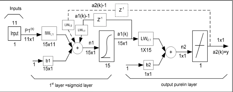
Mathematical relationship among each layer’s content considering transfer function in the proposed Elman and Jordan network structure is illustrated in Figure 2. Note that the feedback connection which is represented by dashed line is for Jordan network.
Figure 2. Elman and Jordan RNN structure applied for training and testing
All calculated values obtained from equation 1, 2, and 13 such as initial weight, layers weight, and bias status is inserted to the structure depicted in Figure 2. For instance, the first layer of Elman network will have the relationship as: a1(k) = logsig(IW1,1.p + LW1,1.a1(k-1)+b1),
whereas the output layer will have a2(k) = purelin(LW2,1.a1(k)+b2). This relationship is then
applied until output is found. Whenever error target is not yet reached, computation will remain continued involving LM algorithm provided in equation 3-12.
structure. The context layer is accomodated with its delay connection for respective layer.In the case of Elman network, it is identified as the first and the second layer, with the feedback connection from the first layer output to the first layer input. Thus, this framework is used in this study.
3.3. Training algorithm and testing mechanism
At each step, input vectors are presented to the network and error is generated. The error is then backpropagated to find gradients of errors for each weight and bias. This approximate gradient is then used to update the weights with the chosen learning function. In the presence of LM learning algorithm, a complete training algorithm for both proposed Elman and Jordan networks is proceeds as follows:
a. Apply preprocessing scheme to scaledown the input and target vector so that they always fall within a specified range of -1 to 1.
b. Create an RNN structure, define network training parameter such as error target and number of epochs.
c. Present all treated inputs and corresponding target output from step 1 to the network. d. Generate initial weights and biases using Nguyen-Widrow method.
e. Compute output of each network, involve feedback form the 1st layer in the case of Elman network or feedback from output layer in the case of Jordan network.
f. Obtain network outputs and errors
V
( )
x
with respect to all inputs.g. Obtain the Jacobian matrix
J
( )
x
.h. Solve Equation (11) to obtain
∆
( )
x
.i. Recompute
V
( )
x
usingx
+
∆
x
. If the newV
( )
x
is less than that computed in step 6, then reduceµ
by some factorγ
, calculatex
+
∆
x
then go to step 6. IfV
( )
x
is not reduced, increaseµ
byγ
, go to step 8.j. The algorithm is completed when
∇
V
( )
x
has reduced to be equal or lower than the predetermined error value.In this paper, two (2) experiments through simulations are presented to obtain the proposed network response in terms of the resulting output changes with respect to different set of input and target training output. The objectives of each experiment are as follows:
a. The first experiment is called base case simulation. The objectives are to justify the network’s structure by obtaining forecasted peak load of 2006-2008 and to compare the result with corresponding actual peak load.
b. The second experiment is carried out to test the network response in terms of producing forecasting peak load of 2009-2011.
Overall, the length of data presented to the network is extended to achieve more accurate result by strengthening network output pattern.
Network performance is defined through a predetermined mean square error (MSE). The error is calculated as the difference between the target output and the network output as given by
∑
=
=
Ni i
e
N
MSE
1 2
1
(14)
Numerical forecasting result is measured in terms of mean absolute percentage error (MAPE) as compared with the actual peak load in the respective year. MAPE is given by
∑
=
−
=
Ni
i i i
N
y
y
y
MAPE
1%
100
.
where
y
i is actual peak load for yeari
, andy
i is forecasting peak load for yeari
,e
is thenetwork’s vector error, and
N
is number of input to the network.4. Result and Discussion
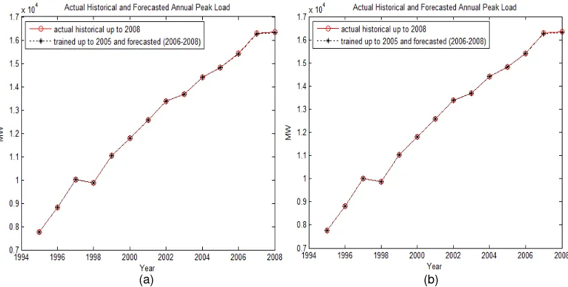
In the first experiment, networks are trained using actual historical data of 1995-2005 and actual historical peak load of 1995-2005 as the network’s input and the training output target, respectively. Afterwards, networks are tested to obtain forecasting peak load for 2006-2008 using projection data of 2006-2006-2008 as the input. In the case of Elman network, the MSE target of 10-5 is reached before the 900th epochs, similarly for the case of Jordan network. Training and forecasting results for the first experiment is shown graphically in Figure 3. The actual historical peak load up to 2008 is depicted using straight line with circle whereas network training during 1995-2005 and forecasting result during 2006-2008 is depicted by dotted line with asterisk.
(a) (b)
Figure 3. Elman (a) and Jordan (b) network’s training and forecasting result, first experiment
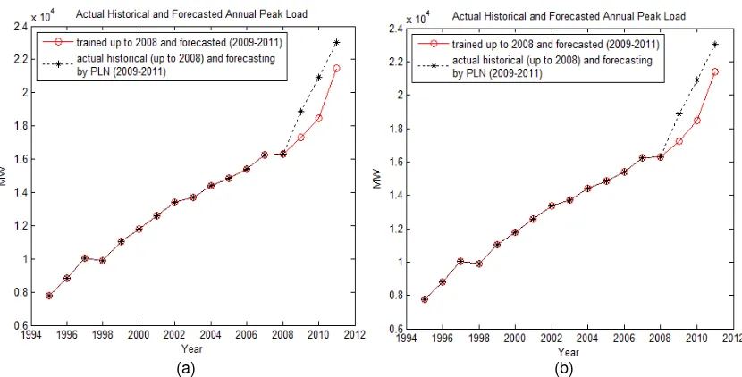
The second experiment is conducted to train the network using actual historical data and peak load of 1995-2008 as input and output target, respectively. Then after, simulation is run to find forecasting peak load for 2009-2011 using projected data set of 2009-2011 as the networks input. The MSE target of 10-5 is reached on the 1031th epochs for Elman network, and for the case of Jordan network is on the 1082th epochs. The actual historical peak load up to 2008 and forecasting peak load by PLN is depicted using dotted line with asterisk whereas network training during 1995-2008 and forecasting result is depicted by straight line with circle.
Figure 3 and Figure 4 give graphical looks on how forecasting result is achieved through the first and second experiment by the proposed networks. It also shows comparison to that available from PLN. In this regards, peak load forecasting by PLN is available from the references [15. 16], in which obtained using econometric approach.
(a) (b)
Figure 4. Elman (a) and Jordan (b) network’s training and forecasting result, second experiment
Table 2. Comparison of forecasting results in MW and MAPE
Year APL
LM-Recurrent Network
LMFN DLMR PLN E1 J1 E2 J2 E3 J3
(Percentage of MAPE compared to actual peak load) 2006 15,402 15,419
(0.11)
15,419 (0.11)
15,434 (0.21)
15,451 (0.32)
15,400 (0.01) 2007 16,259 16,282
(0.14)
16,285 (0.16)
16,297 (0.23)
16,234 (0.15)
16,478 (1.35) 2008 16,309 16,357
(0.29)
16,345 (0.22)
16,347 (0.23)
16,423 (0.70)
17,631 (8.11) 2009 17,211 17,229
(0.10)
17,232 (0.12)
17,269 (0.34)
18,788 (9.16)
18,854 (9.55) 2010 17,890 18,467
(3.22)
18,453 (3.15)
19,508 (9.04)
20,870 (16.66)
20,900 (16.82) 2011 n/a 21,483
(--)
21,420 (--)
21,527 (--)
23,212 (--)
23,012 (--)
As shown in Table 2, peak load forecasting result either by LMFN and DLMR is obtained from [1], whereas forecasting provided by PLN is taken from [15, 16] of which based on econometric approach. From the first experiment symbolized by E1 and J1, both Elman and Jordan network are well trained using 1995-2005 input data and considered perform satisfactory forecasting outputs for 2006-2008 since the average error in terms of MAPE is 0.18% and 0.16%, respectively. Meanwhile, LMFN network error is slightly higher with 0.22%, and followed by DLMR for 0.39%. In addition, the yearly error obtained by the current proposed networks are less than 1% compared to that shown by PLN projection, of which accounted for 3.16%.
selecting factor thought to affect peak load forecasting. In this regards, elasticity and possibility of captive power diversion to the grid are taken into consideration in forecasting made by PLN [16].
It should be noted that the main objective in this research is to compare the capability of selected methods with respect to their forecasting accuracy over the given period. It should be noted that there is difference in forecasting methodology between ANN and econometric approach, of which previously done using DLMR and method by PLN. In case of applying ANN, the immediate concern is to achieve reasonably accurate network training output, which is obtained through having the peak load pattern over the pass period when the network is trained under the specified limited epoch. In this research, MSE is set to 1.10-5 for which the network is expected to be able to provide good pattern for the forecasting purpose as it is succeed for this study. In other words, we can determine how much error we want there in the network to allow it generates a reasonably good pattern. On the other hand, by having the regression result, error produced by the model over the several variables contributes in it can be calculated afterwards. That is why the ANN fitted error for 1995-2008 in term of MAPE or MSE far less than that generated by the regression model. MAPE or MSE of ANN can be practically considered as zero during 1995-2005 for the first experiment and during 1995-2008 for the second experiment.
5. Conclusion
Experiments carried out using the proposed Elman and Jordan networks has been conducted in this research to deal with the long-term peak load forecasting problem for JaMaLi taken into account several factors thought to influence the region’s peak load pattern. The ability of the networks to generate fairly good results are quite satisfactory in terms of low MAPE although within limited forecasting periods, for which the network pattern are strengthened provided a limited training period. Next research may deal with the application of optimization techniques to further strengthen networks pattern and improve results provided limited period of data.
References
[1] Tanoto Y, Ongsakul W, Marpaung COP. Long-term Peak Load Forecasting Using LM-Feedforward Neural Network for Java-Madura-Bali Interconnection, Indonesia. PEA-AIT International Conference on Energy and Sustainable Development: Issues and Strategies. Bangkok. 2010: 1-6.
[2] Kuncoro AH, Zuhal, and Dalimi R. Longterm Peak Load Forecasting on the Java-Madura- Bali Electricity System Using Artificial Neural Network Method. International Conference on Advances in Nuclear Science and Engineering in Conjunction with LKSTN. Bandung. 2007: 177-181.
[3] Kermanshahi B. Recurrent Neural Network for Forecasting Next 10 Years Loads of Nine Japanese Utilities. Neurocomputing.1998; 23: 125-133.
[4] Kermanshahi B, Iwamiya H. Up to Year 2020 Load Forecasting Using Neural Nets. Electrical Power and Energy System. 2002; 24: 789-797.
[5] El-Ela AA. El-Zeftawy AA, Allam SM, Atta GM. Long-term Load Forecasting and Economical Operation of Wind Farms for Egyptian Electrical Network. Electric Power Systems Research. 2009; 79: 1032-1037. [6] Parlos AG, Patton AD. Long-term Electric Load Forecasting Using Dynamic Neural Network
Architecture. Joint International Power Conference Athens Power Tech. Athena. 1993; Volume 2: 816-820.
[7] Lina R, Yanxin L, Zhiyuan R, Haiyan L, Ruicheng F. Application of Elman Neural Network and MATLAB to Load Forecasting. International Conference on Information Technology and Computer Science. Washington DC. 2009; Volume 1: 55-59.
[8] Hagan MT, Menhaj MB. Training Feedforward Networks with the Marquardt Algorithm. IEEE Transactions on Neural Networks. 1994; 5(6): 989-993.
[9] Ghods L, Kalantar M. Methods for Long-term Electric Load Demand Forecasting: A Comprehensive Investigation. IEEE International Conference on Industrial Technology. Chengdu. 2008: 1-4.
[10] Daneshi, H. et al. Long-term load forecasting in electricity market. IEEE International Conference on Electro/Information Technology. Ames. 2008 Page(s):395 – 400.
[11] Tanoto Y. Long-term Peak Load Forecasting Using Artificial Neural Networks: The Case of Java-Madura-Bali Interconnection, Indonesia. Master Thesis. Bangkok, Asian Institute of Technology; 2010. [12] Nguyen D, Widrow B. Improving The Learning Speed of 2-Layer Neural Networks by Choosing Initial Values of The Adaptive Weights. The International Joint Conference on Neural Networks. San Diego.1990; Volume 3: 21-26.
[14] Jadid MN, Fairbairn DR. Predicting Moment-Curvature Parameters from Experimental Data.
Engineering Application Artifical Intelligence.1996; 9(3): 303-319.
[15] PT. PLN (Persero). National Electricity Planning and Provision (RUPTL 2006-2015–in Bahasa Indonesia). Jakarta. 2006.
![Figure 1. Elman and Jordan Recurrent Neural Networks architecture [11]](https://thumb-ap.123doks.com/thumbv2/123dok/247782.503905/2.595.139.459.460.659/figure-elman-jordan-recurrent-neural-networks-architecture.webp)