DOI: 10.12928/TELKOMNIKA.v15i1.4510 314
Diurnal Variability of Underwater Acoustic Noise
Characteristics in Shallow Water
Yasin Yousif Al-Aboosi*1, Abdulrahman Kanaa2, Ahmad Zuri Sha'ameri3, Hussein A. Abdualnabi4
1,2,3Faculty of Electrical Engineering, Universiti Teknologi Malaysia, 81310, Johor, Malaysia
1,4
Faculty of Engineering, University of Mustansiriyah, Baghdad, Iraq *Corresponding author, e-mail: [email protected]
Abstract
The biggest challenge in the underwater communication and target locating is to reduce the effect of underwater acoustic noise (UWAN). An experimental model is presented in this paper for the diurnal variability of UWAN of the acoustic underwater channel in tropical shallow water. Different segments of data are measured diurnally at various depths located in the Tanjung Balau, Johor, Malaysia. Most applications assume that the noise is white and Gaussian. However, the UWAN is not just thermal noise but a combination of turbulence, shipping and wind noises. Thus, it is appropriate to assume UWAN as colored rather than white noise. Site-specific noise, especially in shallow water often contains significant non-Gaussian components. The real-time noise segments are analyzed to determine the statistical properties such as power spectral density (PSD), autocorrelation function and probability density function (pdf). The results show the UWAN has a non-Gaussian pdf and is colored. Moreover, the difference in UWAN characteristics between day and night is studied and the noise power at night is found to be more than at the day time by around (3-8dB).
Keywords: underwater acoustic noise, colored noise, non-gaussian statistics
Copyright © 2017 Universitas Ahmad Dahlan. All rights reserved.
1. Introduction
Where f is the frequency in kHz. The total noise power spectral density for a given frequency f [kHz] is then:
(5)
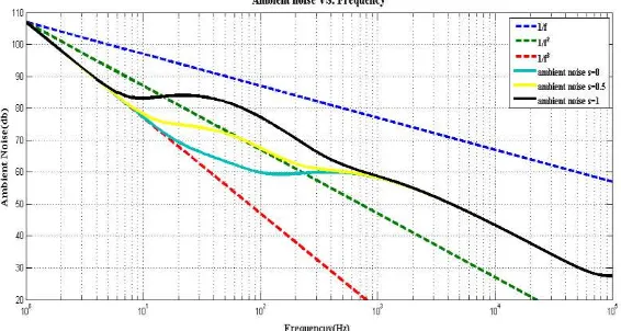
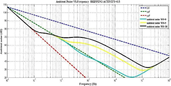
Figure 1 illustrates the empirical noise PSDs for different levels of shipping activities and with a wind speed of 3.6 m/sec (7 knots). Figure 2 shows the empirical noise power spectrum densities for different conditions of wind speed and with shipping activities (S=0.5). In general, the UWAN power spectrum is located in the area between the two curves ( ) and ( ). Moreover, it can be observed the turbulence noise is dominant in the frequency band (0.1Hz - 10Hz), while shipping activities are the major contributors to noise in a higher frequency band (10Hz - 200Hz). Shipping activities are usually weighted by a factor s which ranges from 0 to 1 which weighs the activity level from low to high activity respectively. The frequency band (0.2 kHz - 100 kHz) is conquered by surface motion, which is primarily affected by wind (w is the wind speed in m/s). For frequencies higher than (100 kHz) thermal noise is dominant. However, these noise sources are highly dependent on weather and other environmental factors.
The UWAN in shallow water has a greater variability in both time and location deep water. Therefore, it is more challenging to model or predict. Typical shallow-water environments cover water depths down to 200m while typical deep-water environments in all oceans are considered at depths exceeding 2000m [8]. In [5, 6], three major noise sources in shallow water environments namely wind noise, biological noise (especially noise created by snapping shrimp whose noise signature has a high amplitude and wide bandwidth) and shipping noise are identified. Furthermore, the UWAN power also decreases with the increasing depth as the distances between the surface, the shipping and wind noises become larger. In general, the UWAN has been shown to be 9 dB higher in shallow water compared to deep water [7].
Figure 1. The noise PSDs in dB re μ Pa per Hz based on empirical formulae with wind speed 3.6 m/s (7 knots) and different Shipping noise is presented for high (s = 1), moderator (s = 0.5),
Figure 2. The noise PSDs in dB re μ Pa per Hz based on empirical formulae with Shipping activity S= 0.5 and for different wind speeds (w =0, 5 and 10 m/s)
3. Statistical Properties and Estimation
Unlike deterministic signals, random signals are best characterized by their statistical properties. Thus, the statistical properties such as autocorrelation function, PSD and pdf are demonstrated in this work.
3.1. Auto-Correlation Function
A random signal can be characterized in terms of the auto-correlation function. It shows the dependency of the signal at one-time t with respect to its time-shifted version by . This is termed as auto-correlation function, which is also the cross-correlation of a signal with itself [9, 10] and is presented as follows:
(6)
Where E[ ] is the expectation operator. If the random process is wide sense stationary, the autocorrelation function can be expressed as:
(7)
The function depends on only relative time rather than the absolute t. In the normalized
case , zero indicates no dependency and one refers to strong dependency [11].
3.2. Power Spectrum Density (PSD) and Estimation
The frequency representation of a random process is known as PSD while the estimation of the PSD is termed power spectrum estimation (PSE). In general, there are two types of (PSE) method: parametric and nonparametric. Unlike parametric PSE, nonparametric PSE does not make any assumption on the data generating process. The relationship between the autocorrelation function and the PSD is defined by the Wiener-Khinchine theorem [10], [12-13].
(8)
(9)
Power spectrum in Equation (8) evaluated at f=0 yields:
(10)
compute a modified periodogram of each segment, then averaging the PSD estimate is performed. The averaging effect introduced in this method decreases the variance in the PSD estimate with further reduction in variance by overlapping of segments.
If the signal is sampled at a normalized sampling frequency, the Welch method [12] can be expressed as:
(12)
Where K is the number of segments, and L is the length of each segment. The normalization factor is:
(13)
Where D is the offset between two consecutive segments.
3.3. Probability Density Function (pdf):
The standard model of noise is Gaussian, additive, independent at each pixel and independent of the signal intensity. In applications, Gaussian noise is most usually used as additive white noise to yield AWGN [9, 14]. It has shaped probability distribution function given by:
(14)
Where μrepresents the mean value and the standard deviation.
Several publications have reported UWAN does not follow the normal distribution. Instead, it follows pdf with extended tails shape, reflecting an accentuated impulsive behavior due to the high incidence of large amplitude noise event [5]. The noise follows the alpha-stable PDF where the characteristic equation has an inverse. Without knowledge of pdf in a closed form, the only solution is to use numerical methods. An alternative modeling method is by means of empirical analysis of the noise samples obtained directly from the underwater environment [15].
The Student's t-distribution is associated with the Gaussian distribution and is characterized by wider tails. It is used in the estimation of the population mean for a small number of samples and unknown population standard deviation. The Student’s t pdf is expressed by [16]:
(15)
Where Γ(·) is the gamma function , is the degree of freedom which controls the dispersion of
the distribution and is the mean value. The lower the value of , wider the tails of the pdf
a) It has mean = 0 and the standard deviation is greater 1 for degrees of freedom, greater than 2 and it does not exist for 1 and 2 degrees of freedom. For sufficiently large values of the degree of freedom, the Student pdf converges to the Gaussian distribution.
b) The mean of is for and does not exist for ; c) The variance of is
for and does not exist for .
4. Results and Discussion
The UWAN samples were obtained directly from the underwater environment. Five different segments of samples were collected diurnally through the experiments conducted in shallow water at Tanjung Balau, Johor, Malaysia (Latitude 1° 35.87'N) and (Longitude 104° 15.793'E) on 22nd March 2014. The segments were received through a broadband hydrophone (7 Hz ~ 22 kHz) model DolphinEAR 100 Series, at different depths from 1 to 5 meters with sea floor at a depth of 10 meters. During the day time, the wind speed was about 8 Knots and the temperature at the surface of the sea about 26 C0 while at night wind speed was about 11 Knots and the temperature at the surface of the sea about 27 C0. The power spectrum is estimated using Welch modified periodogram technique and the data were analyzed for various depths. The setup for the power spectrum estimation is as follows: sampling frequency 8kHz, window type Hanning, 2048-point fast Fourier transform (FFT), FFT window size of 256 samples and 50% overlapping. Figure 3 shows the experiment site.
Figure 3. Experiment Test Site
Figure 4. Field Trials Conducted at Tanjung Balau, Johor, Malaysia on the 22nd March 2014.
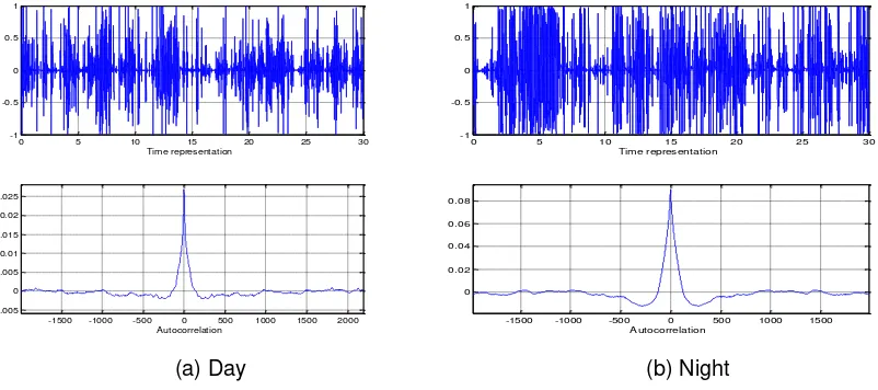
Figure 5 shows the time representation waveform and the autocorrelation function of the collected data during the day and night with depths of 3 meters Unlike white Gaussian noise, the biased autocorrelation function is not similar to the unit impulse which means that the noise samples are correlated and considered colored. The value of the autocorrelation function
at =0 represented the noise power Shows clearly the noise power at night is more than at day.
(a) Day (b) Night
Figure 5. Time Representation Waveform and Autocorrelation Function of the Underwater Acoustic Noise for the Day and Night at Depth 3 Meters
1 meter depth 2 meters depth
Figure 6. Welch PSD Estimate of UWAN for the Day and Night at Two Different Depths of 1 meter and 2 meters.
-1500 -1000 -500 0 500 1000 1500 2000 -0.005
-1500 -1000 -500 0 500 1000 1500 0
0 500 1000 1500 2000 2500 3000 3500 4000
-80
0 500 1000 1500 2000 2500 3000 3500 4000
(a) Day
(b) Night
Figure 7. Welch Noise PSD estimate of UWAN for the day and night at depth 3 meters in logarithm scale
(a) day (b) night
Figure 8. Comparison of the amplitude distribution of the UWAN with the Gaussian distribution and t-distribution for the day and night at depth 3 meters
5. Conclusion
[1] AG Borthwick. Marine Renewable Energy Seascape. Engineering. 2016; 2: 69-78.
[2] M Stojanovic, J Preisig. Underwater acoustic communication channels: Propagation models and
statistical characterization. Communications Magazine, IEEE. 2009; 47: 84-89.
[3] T Melodia, H Kulhandjian, LC Kuo, E Demirors. Advances in underwater acoustic networking. Mobile
Ad Hoc Networking: Cutting Edge Directions. 2013: 804-852.
[4] RP Hodges. Underwater acoustics: Analysis, design and performance of sonar. John Wiley & Sons. 2011.
[5] M Chitre, JR Potter, SH Ong. Optimal and near-optimal signal detection in snapping shrimp
dominated ambient noise. Oceanic Engineering, IEEE Journal of. 2006; 31: 497-503.
[6] RJ Urick. Ambient noise in the sea. DTIC Document. 1984.
[7] G Burrowes, JY Khan. Short-range underwater acoustic communication networks. INTECH Open Access Publisher. 2011.
[8] WM Hartmann. Signals, sound, and sensation (Modern Acoustics and Signal Processing). AIP Press. 1996.
[9] AM Yaglom. Correlation theory of stationary and related random functions: Supplementary notes and references. Springer Science & Business Media. 2012.
[10] AV Oppenheim, GC Verghese. Signals, systems, and inference. Class notes. 2010; 6.
[11] F Hooge. 1/f noise. Physica B+C, 1976; 83: 14-23.
[12] HR Gupta, S Batan, R Mehra. Power spectrum estimation using Welch method for various window
techniques. International Journal of Scientific Research Engineering & Technology. 2013; 2: 389-392.
[13] CW Therrien. Discrete random signals and statistical signal processing. Prentice Hall PTR. 1992. [14] PZ Peebles, J Read, P Read. Probability, random variables, and random signal principles vol. 3. New
York: McGraw-Hill. 2001.
[15] J Panaro, F Lopes, LM Barreira, FE Souza. Underwater Acoustic Noise Model for Shallow Water
Communications. In Brazilian Telecommunication Symposium. 2012.
[16] AZ Sha'ameri, Y Al-Aboosi, NHH Khamis. Underwater Acoustic Noise Characteristics of Shallow
Water in Tropical Seas. In Computer and Communication Engineering (ICCCE), International Conference on. 2014: 80-83.