Local Model Checking Algorithm Based on Mu-calculus with Partial Orders

DOI: _{10.12928/TELKOMNIKA.v15i1.3546}  ₄₂₁

Local Model Checking Algorithm Based on Mu-calculus

with Partial Orders

Hua Jiang*1, Qianli Li2, Rongde Lin3

1,2

Key Lab of Granular Computing, Minnan Normal University, Zhangzhou 363000, Fujian, China 3_{School of Mathematical Science, Huaqiao University, QuanZhou 362021, Fujian, China}

*Corresponding author, e-mail: sg_jh@126.com

Abstract

The propositionalμ-calculus can be divided into two categories, global model checking algorithm and local model checking algorithm. Both of them aim at reducing time complexity and space complexity effectively. This paper analyzes the computing process of alternating fixpoint nested in detail and designs an efficient local model checking algorithm based on the propositional μ-calculus by a group of partial ordered relation, and its time complexity is O(d2(dn)d/2+2) (d is the depth of fixpoint nesting,

n

is the maximum of number of nodes), space complexity is O(d(dn)d/2). As far as we know, up till now, the best local model checking algorithm whose index of time complexity is d. In this paper, the index for time complexity of this algorithm is reduced from d to d/2. It is more efficient than algorithms of previous research.

Keywords: model checking, propositional mu-calculus, computational complexity, fixpoint, partitioned dependency graph

Copyright © 2017 Universitas Ahmad Dahlan. All rights reserved.

1. Introduction

Propositional



-calculus [1-4] model checking technique is widely used in the design and verification of the finite-control concurrent system. Model checking algorithms can be segmented into two categories. One is global model checking that obtains all the sets of states which satisfy a given logic expression in a finite-control concurrent system. The other is local model checking, which is not always necessary to examine all the states. As we know, the state space explosion problem is the main problem that the propositional



-calculus model checking algorithm faces with, so it is one of the hot topics to reduce time complexity and space complexity effectively.

For global model checking, according to Tarski Fixpoint theory [5] and the fixpoint operator of formula, it can be computed by iteration. A number of global algorithms have been devised, for global propositionalμ-calculus, Emerson and Lei [6] presented a global algorithm that time complexity of the global algorithm was

O n

(

d1

)

, then Andersen, Cleaveland and Steffen, et al., [7] improved the algorithm in [6], but the time complexity was still

O n

(

d1

)

. In 1994, Long, Browne and Clarke, et al., [10] got a group of partial ordered relation by Tarski fixpoint theory and designed a global algorithm, both time complexity and space complexity were

O n

(

d/2 1

)

. In 2010, Hua Jiang [11] got two groups of partial ordered relation by Tarski fixpoint theory and designed a global algorithm, the time complexity of the global algorithm was

/2 1

((2

1)

d

)

O

n



 , and the space complexity is

O dn

(

)

, at present, this is the best study result of global model checking algorithm. Because the global algorithms can not solve some practical problems perfectly, the local model checking was necessary.

alternating fixpoints. Though reference [17] improved the complexity of the local algorithm, its efficiency did not achieve the desired results.

Related work can be found in [19] which presented global and local algorithms for computing fixpoint in linear time. In this way, the occurrence of the state exponential explosion problem is delayed, global algorithm is compared with local algorithm in [20], Jiang Hua [21] described an improved algorithm of global model checking for propositional μ-calculus. Modal μ -calculus are also important for studying probabilistic systems, Liu Wangwei, et al., [22] presented a natural and succinct probabilistic extension of μ-calculus, called PμTL, Castro Pablo, et al, [23] presented a probabilistic μ-calculus by using probabilistic quantification as an atomic operation and showed that PCTL and PCTL* can be captured in μ-calculus.

In this paper, we obtain a group of partial order relation by Tarski Fixpoint theory and the fixpoint operator of formula, then we present the bound algorithm which is based on the group of partial order relation. In this way, we can reduce the complexity and improve the computational efficiency. Our main result is a new efficient local algorithm that makes extensive use of monotonicity considerations to reduce the complexity of evaluation for evaluating partitioned dependency graphs [15] fixpoints. And the index for time complexity of this algorithm is reduced from

d

to

d

/ 2

.

The structure of the rest of this paper is organized as follows. In section 2, the equivalence between semantics of propositionalμ-calculus and Partitioned Dependency Graphs(PDGs) is introduced, and the basic algorithm for evaluating PDG fixpoint is analyzed in detail. Section 3 gives the partial order relation in the evaluating PDG fixpoint firstly, and then presents a new algorithm based on partial orders, shows the time and space complexity of the algorithm is

O d

(

2



(

dn

)

d/2 2

)

and

O d dn

(



(

)

d/2

)

, and finally gives some experimental results. This paper ends with a detailed discussion of some conclusions and directions for future research in section 4.

2. Partitioned Dependency Graphs and Fixpoint Evaluating Algorithm

The syntax of propositional μ-calculus formulas and the semantics under the transition system are refer to [24]. To guarantee the existence of the fixpoints, formulas with positive normal form (PNF) [1] are considered only, where each propositional variable is restricted to a fixpoint operator at most and the operator



only acts on the atomic proposition.

2.1. Partitioned Dependency Graphs

Let transition system

M



( , , )

S T L

, where

S

is a non-empty set of states,

L

is a

mapping each atomic proposition to a subset of

S

, and

T

maps

 

a

{ , , ,

a b a a

_{1 2}

,...}

to a tuple of state,

T a

:



( , )

S S

. For given a PNF fixpoint formula

 

R

.

or

 

R

.

, the semantics

denotes as

.

( )

M

R

S

 

or

.

( )

M

R

S

 

respectively, which is the least fixpoint or greatest fixpont of the predicate transformer respectively. So the mapping between two subset of states defined by predicate transformer is a dependency, and thus the computation sequences of fixpoint evaluatings is equivalent to a partitioned dependency graphs [15].

Definition 1. A partitioned dependency graph ( PDG ) is a tuple

( , , ... , )

V E V V

_{1 n}



, where

V

is a set of vertices,

E

 

V

2

V is a set of hyper-edges,

V V

₁

...

_n is a finite sequence of subsets of

V

such that

{ ,..., }

V

₁

V

_n is a partition of

V

, and



:{ ,..., }

V

₁

V

_n



{ , }

 

is a function that assigns



or



to each block of the partition [15]. Let

  



{ , }

. We shall

subsequently write



( )

x





if

x V



i and



( )

V

i





.

G

is a

PDG

,

G



( , , ... , )

V E V V

_{1 n}



. Xinxin Liu, et al., [15] regarded

G

as a nested boolean equation system [13],

 

x V x

i

,

 

( , )x SE



y S

y

. And



( )

V

i are nested in

V V

1

...

n,

Example 1.

G

is a

PDG

and

G



( , ,

V E VV VV

_{1 2 3 4}

, )



, where

1 2 3 4 5 6

{ , , , , , }

V



x x x x x x

,

V

₁



{ , }

x x

_{1 2} ,

V

₂



{ }

x

₃ ,

V

₃



{ , }

x x

_{4 5} ,

V

₄



{ }

x

₆ ,

1 3 4 2 6 2 5 3 1 5 4 1 5 3 6 6 1

{( ,{ , }),( ,{ }),( ,{ }),( ,{ , }),( ,{ }),( ,{ , }), ( ,{ }),

E



x x x

x

x

x

x

x x x

x

x

x

x x

x

x

( ,{ })}

x x

6 4 ,

1

( )

V







,



( )

V

₂





,



( )

V

₃





,



( )

V

₄





. Thus, the corresponding nested boolean equation system consists of:

1 3 4 2 5 6

=x

:

x

x

v

x

x

x





  



,



:{

x

3

 

x

1

x

5,

4 1 5 3 6

=x

:

x

v

x

x

x



  



,



:{

x

6

 

x

1

x

4

2.2. Algorithm for PDG fixpoint Evaluatings

In reference [15] a local algorithm for evaluating PDG fixpoint, namely LAFP is proposed, where the search space is constructed as a subset of

V

which is divided into three blocks, and computes the fixpoints iteratively.

Given a PDG, let

b

denote the out-to-in sequence

b b

₁

, ,...,

₂

b

_d, where

d

(

d

mod 2



0

) is fixpoint nesting depth. There are

n

_i nodes in

b

_i, and the fixpoint types are

2k 1

(

V

2k 1

)



 





,



2k

(

V

2k

)





,

k



1, 2,...

, respectively. So all the sequences of

b

are as

follows:

0

1

( 1)

1 1 10 11 1 1 1

2 2 20 21 2 2 2

1 1 ( 1)0 ( 1)1 ( 1) 1 1 0 1

:

{

,

,...,

},

( )

:

{

,

,...,

},

( )

:

{

,

,...,

},

(

)

:

{

,

,...,

d n n

d d d d d n d d

d d d d dn

b V

x

x

x

V

b V

x

x

x

V

b

V

x

x

x

V

b V

x

x

x













       















},

(

)

d



d

V

d























(1)

Let’s divides

V

i into three blocks, denoting

' '' '''

i i i i

V

  

V

V

V

(1

 

i d

)

, where

V

_i'

saves nodes waiting for computing,

V

_i''saves nodes which have been identified,

V

_i''' saves

nodes which have not been identified. A assume that the initial value of state of each node of

V

_i are

True

or

False

, then

V val

₁

(

)



True

,

V val

₂

(

)



False

,

V val

₃

(

)



True

,

4

(

)

V val



False

, …,

V

d1

(

val

)



True

,

V val

d

(

)



False

respectively,

V val

i

(

)

means the

initial value of state of each node.

Let

g g

₁

,

₂

,...,

g

_d1

,

g

_d be the computation function of the corresponding node of

b

in PDG, then the iteration formulas is as follows:

1 1 1 1 1

1 2 1 1 2 1 2 1 2

1 2 1 1 1 2 1 2 1 1 2 1

1 2 1

1 ... ...

1 1 1 2 1

( 1) ... ..

2 2 1 2 1

...( 1) ... ...

1 1 1 2 1

... ( 1)

1

(

,

,...,

,

)

(

,

,...,

,

)

(

,

,...,

,

)

(

d d d

d d

k k k k k

d d k k k k k k k k k

d d

k k k k k k k k k k k k

d d d d

k k k k

d d

V

g V

V

V

V

V

g V

V

V

V

V

g

V

V

V

V

V

g V

                    









1 1 2 1 2... 1 1 2... 1

2 1

,

,...,

k k kd

,

k k kd kd

)

k k k

d d

V

V



V



 ₍₂₎

1

.

1

V val



V

,

V val

₁

.

means the iteration value of the nodes of

V

₁. When 1

1

.

1

k

V val



V

, then the

computation sequence of

V

₂ is 10 11 12 1( 1) 1

2

,

2

,

2

,...,

2

,

2

k k k k k

V

V

V

V



V

. When 1

1

.

1

k

V val



V

,

1 2

2

.

2

k k

V val



V

, then the computation sequence of

V

₃ is 1 20 1 21 1 22 1 2( 1) 1 2

2

,

2

,

2

,...,

2

,

2

k k k k k k k k k k

V

V

V

V



V

.

When 1

1

.

1

k

V val



V

, 1 2

2

.

2

k k

V val



V

,…, 1 2... 1

1

.

1

d k k k

d d

V

val

V







 , then the computation sequence of

d

V

is k k1 2...kd10

,

k k1 2...kd11

,

k k1 2...kd12

,...,

k k1 2...kd1( 1)

,

k k1 2...kd1

d d d d d

V



V



V



V

 

V

_.

Therefore we can obtain k k1 2...k ki1i 'k k1 2...k ki1i ''k k1 2...k ki1i '''k k1 2...k ki1i

i i i i

V





V





V





V

 _.

Thus, for given a PDG, the nesting computation sequence of Equation (1) descripted as:

00...00 00...01 00...02 00...0 00...1 00...10 00...11 00...12 00...1 00...2

1 1

,

,

,...,

,

,

,

,

,...,

,

,

d d d d d d d d d d

V

V

V

V



V

_

V

V

V

V



V

_

00...( 1)0 00...( 1)1 00...( 1)2 00...( 1) 00... 01

1 2

01...00 01...01 01...02 01...0 01...1 01...10 01...11 01...12 01...1 01...2

1 1

,

,

,...,

,

,...

,

,

,

,...,

,

,

,

,

,...,

,

,

d d d d d

d d d d d d d d d d

V

V

V

V

V

V

V

V

V

V

V

V

V

V

V

V

               (3)

01...( 1)0 01...( 1)1 01...( 1)2 01...( 1) 01... 02 0 1

1 2 2 1

10...00 10...01 10...02 10...0 10...1 10...10 10...11 10...12 10...1 10..

1 1

,

,

,...,

,

,...

,...,

,

,

,

,

,...

,

,

,

,

,...

,

d d d d d

d d d d d d d d d d

V

V

V

V

V

V

V

V

V

V

V

V

V

V

V

V

V

V

      

 

   



 .2

,

10...( 1)0 10...( 1)1 10...( 1)2 10...( 1) 10... 11 11...00 11...01 11...0

1 2

11...1 11...10 11...11 11...12 11...1 11...2 11...

1 1 1

,

,

,...,

,

,...

,

,

,...,

,

,

,

,

,...,

,

,...,

,

d d d d d d d d

d d d d d d d

V

V

V

V

V

V

V

V

V

V

V

V

V

V

V

V

      

 

   



  

...

V

212

,...,

V

21

,

V

12

,...,

V

1

 

3. Local Model Checking Algorithm based on Partial Orders 3.1. Partial Ordering Relation of Computing Node Set

Let _{( , , )} i

val i r

N

_ denotes data structure of computing nodes of

V

,

r

_i

(1

 

r

_i

n

_i

)

is free variable,

val



{

True False

,

}

,

  



{ , }

,

i

is nesting level. We will superscript relation names

with vectors of iteration indices to show various approximations. We will let

k

_i

(0

 

k

_i

n

)

and

i

k

denote vectors of iteration indices. For example, ki0

i

V

denotes k k1 2... 0ki i

V

,

k

i

0



k k

1 2

... 0

k

i . If

0

00...00

i

k



, then ki0

i

V

means

V

_i00...00. The notation

Cas k

( )

_t means that

k

_t is the closest

antecedent sequence. That is to say, if

k

_t

h

_t, and

  

h

_i

k

_i

1

, where

1

 

i

t

, then we have

( )=

_{t t}

Cas h

k

.

Let

A

and

M

be node sets which consist of _{( , , )}

(1

)

i

val i r

N

_

 

i d

, and satisfy both of the

following criteria, (1)

| | = |

A

M

|

. (2) if _{( , , )} i

False i r

N

_



A

, then _{( , , )} i

True i r

N

_



A

. if _{( , , )} i

True i r

N

_



A

, then

( , , )i

False i r

N

_



A

；

M

is similar. where _{( , , )} i

val i r

N

_ is the data structure of computing nodes and

(1

)

i i i

r

 

r

n

is free variable.

Definition 2.

F(A,M ) = A M

is one-way, if

A

and

M

satisfy both of the following criteria

(1)

_{( , , ) ( , , ) ( , , )}

i i i

False False True

i r i r i r

N

_

N

_

N

_



 

A



M





M

.

(2)

_{( , , ) ( , , )}

i i

True True i r i r

N

_

N

_

Clearly,

F

satisfies reflexive, antisymmetrical and transitive, that is to say,

F

is a partial ordering relation of computing node set.

For the iteration formulas (2), when 1

1

.

1

k

V val



V

, 1 2

2

.

2

k k

V val



V

,…, 1 2... 1

1

.

1

d k k k

d d

V

val

V









, then the computation sequence of

V

_dis

1 2...d10

,

1 2...d11

,

1 2...d12

,...,

1 2... d1( 1)

,

1 2... d1

k k k k k k k k k k k k k k k

d d d d d

V



V



V



V

 

V

_；

Because



_d

( )

V

_d





, the

val

of each node of

V

_d is

False

or

True

. If

val

is changed from

False

to

True

, then storing the corresponding node of

val

in

V

_d''. If

1 2...d10

,

1 2...d11

,

1 2...d12

,...,

1 2...d1( 1)

,

1 2...d1

k k k k k k k k k k k k k k k

d d d d d

V



V



V



V

 

V

 _{never change, by the Definition 4.2,} the sequence satisfies the formulas

F

, that is to say, the sequence is one-way, at the same

time,

g g

₁

,

₂

,...,

g

d₁

,

g

d is monotonous, then:

1 2...d10 1 2...d11 1 2...d12

...

1 2...d1( 1) 1 2...d1

k k k k k k k k k k k k k k k

d

V

d

V

d

V

d

V

d

V

d

 

     

F :

；

For



d₁

(

V

d₁

)





, we have:

1 2... 2 1 2... 2( 1) 1 2... 2( 2) 1 2... 21 1 2... 20

1 1 1 1

...

1 1

d d d d d

k k k k k k k k k k k k k k k

d

V

d

V

d

V

d

V

d

V

d

  

      

     

F

:

； (4)

For



₂

( )

V

₂





, we have 10 11 12 1( 1) 1

2 2 2 2

...

2 2

k k k k k

V

V

V

V



V



F :

；

For



₁

( )

V

₁





, we have

F :

₁

V

₁

V

₁(1)

V

₁(2)

...

V

₁1

V

₁0.

Definition 3.

k k

_{1 2}

...

k

_t and

h h h

_{1 2}

...

_t are non-negative integer sequence, and both of them have

t

integers.

k k

_{1 2}

...

k

_t is antecedent than

h h h

_{1 2}

...

_t, if they satisfy both of the following criteria:

(1) Exiting an odd (even) bit

j

of

k k

_{1 2}

...

k

_t and

h h h

_{1 2}

...

_t, s.t.

k

_j



h

_j, where

1

 

j t j

, mod 2



0

.

(2)

k

_m



h

_m, where

1

 

m t

,

m



j

；

1 2

...

t

k k

k

is antecedent than

h h h

_{1 2}

...

_t, denoted

k k

_{1 2}

...

k

_t

h h h

_{1 2}

...

_t；

k k

_{1 2}

...

k

_t 1 2

...

t

h h h

denotes that k k1 2...kt i

V

has been computed when h h1 2...ht i

V

is computed.

Definition 4.

k k

_{1 2}

...

k

_t is the antecedent sequence of

h h h

_{1 2}

...

_t, if they satisfy both of the following criteria:

(1)

k k

_{1 2}

...

k

_t

h h h

_{1 2}

...

_t. (2)

  

h

_i

k

_i

1

, where

1

 

i

t

；

1 2

...

t

k k

k

is the closest antecedent sequence of

h h h

_{1 2}

...

_t, denoting

Cas h h h

(

_{1 2}

... )

_t =

1 2

...

t

k k

k

.

Lemma 1 If

 

_i



,

Cas h h h

(

_{1 2}

... )

_t =

k k

_{1 2}

...

k

_t, then h h1 2...hi i

V

and k k1 2...ki i

V

satisfy

F

,

denoting h h1 2...hi i

V

k k1 2...ki i

V

. Proof. (abbreviated)

Definition 5.

k k

_{1 2}

,...,

k

_t is an generalized antecedent sequence of

h h

_{1 2}

,...,

h

_t, if they satisfy both of the following criteria:

sequence of

h h

_{1 2}

,...,

h

_t satisfy the lexicographic order, denoting

1 2 1 2

( (

,..., ))

_t

( (

,..., ))

_t

lo os k k

k

lo os h h

h

.

1 2

,...,

t

k k

k

is an generalized antecedent sequence of

h h

_{1 2}

,...,

h

_t, denoting

( )

_{t t}

Gas h



k

, where

k

_t is

k k

_{1 2}

,...,

k

_t and

h

_t is

h h

_{1 2}

,...,

h

_t. Lemma 2. If

 

_i



,

Gas h

( )

_t



k

_t, then ki

i

V

and hi

i

V

satisfy

F

, denoted hi ki

i i

V

V

.

Proof. (abbreviated)

3.2. Local Model Checking Algorithm based on Partial Orders

As described above, LAFP presents an efficient local model checking algorithm, however, in the nested process, inner value of fixpoint is affected by outer value of fixpoint. If the value of outer iteration does not change, then the outer value of fixpoint starts computing with the value of inner iteration. When the value of outer iteration is changed, then all the inner value need to update, that is to say, a lot of computing processes is repeated.

For arbitrary sequence

k

_i,

i

mod 2 = 1, by Lemma 1 and Lemma 2, we only need to start the computing from the antecedent sequence

Cas k

( )

_i without affecting the correctness of

result. Thus, let ki Cas k( )i

i i

V



V

instead of ki

i

V



True

, then the iteration time can be reduced and the computing efficiency can be improved. The Local Model Checking Algorithm based on Partial Orders is as follows:

Algorithm 1 Local Model Checking Algorithm based on Partial Orders 1. for ( i = 1; i <= d; i ++ ) do

2.

V

_i'



V

_i

，

V

_i''

 

，

V

_i'''

 

；

// initialize 3. end for

4. i = d; // begin to compute from the innermost layer 5. while ( i > 0 ) do

6. if ( i == d ) then 7. Do

8. dequeue a node

V

_i* from

V

_i';

9.

V

_i'

 

V

_i'

V

_i*; //remove

V

_i*

10. 1 1 1 1 1 1

1 1 1

(

,...,

,

,

)

i i i i i i i

k k k k k k k n

i i i i i

V



g V

V

V

V



 

- -

-=

;

11. if ( val of ki1ki 1

i

V

-  _{changed ) then}

12.

V

_i''



V

_i''



V

_i*;

13. else

V

_i''



V

_i''



V

_i*; 14. end if

15. until

V

_i'

 

; 16. i = i -1; 17. end if

18. if ( i != d ) then 19. Do

20. dequeue a node

V

_i* from

V

_i';

21.

V

_i'

 

V

_i'

V

_i*;

22. 1 1 1 1 1 1

1 1 1

(

,...,

,

,

)

i i i i i i i

k k k k k k k n

i i i i i

V



g V

V

V

V



 

- -

-=

;

23. if ( val of ki1ki 1

i

V

-  _{changed ) then}

25. for ( t > i && t <= d ) do // update the value of all the inner layer 26. if ( t % 2 == 0 ) then

27. kt0

t

V



False

; // the initial value is False

28. else if (

os k

( 0)

_i



0

) then 29. kt0

t

V



True

; // the initial value is True

30. else kt0 Cas k( )t

t t

V



V

; //the initial value is Cas k( )t

t

V



31. end if 32. end if 33. end for

34. else

V

_i''



V

_i''



V

_i*; 35. end if

36. until

V

_i'

 

; 37. i = i – 1; 38. end if 39. end while

3.3. Time Complexity Analysis

When

i



1

, according to 3.2, the computation sequence of the corresponding node is

0 1 2 1

,

1

,

1

,...,

1

V V V

V

 in block

b

₁,

n

₁ is the total number of computing node of block

b

₁. The initial

value of

val

is

True

in each node by



₁

( )

V

₁





. When the value of

val

turns into

False

from

True

, by the monotonicity of function

g

₁, the value of the node no longer changes in the

whole computing process, so the node is deposited in

V

₁''. The worst case is that the value of

val

turns into

False

from

True

after computing each node of

V

1', so the greatest computing

times of corresponding node in block

b

₁ are

|

g

₁

| 1 2 ...

    

n

₁

n

₁2.

When

i



2

,

V val

₁

.

= 1

1

k

V

, the computation sequence of the corresponding node is

10 11 12 1

2

,

2

,

2

,...,

2

k k k k

V

V

V

V

 in block

b

₂, the computing times of the corresponding node are

2

1 2 3 ...

   

n

in block

b

₂, the number of different values of

V val

₁

.

is

n

₁, so the greatest computing times of corresponding node in block

b

₂ are

|

g

₂

|



n

₁

(1 2 3 ...

   

n

₂

)

 

n n

_{1 2}2.

When

i



3

, according to Algorithm 1, if

k

₁



0

,

k

₃



0

,

V

₃ starts to compute from

V

₃'. In this case, the times are

n

₂ at most. The changing times of corresponding node value are

2 3

n n



in block

b

₃, and the computing times are not more than

n n

2 32. When

k

1



0

,

k

3



0

,

V

3

starts to compute from 1 2 3

3

x x x

V

. In this case, the times are

n n

_{1 2} at most, when it reaches the fixpoint, the computing times are

n n n

_{1 2 3} at most, so the greatest computing times of corresponding node in block

b

₃ are

|

g

3

|

    

n n

2 32

n n n

1 2 3.

Summarily, when

i



2

,

|

g

2i

|



n n n

2 4 6

...

n

2i2 2 1 2

n

i

n

2i,

2

2 1 2 4 6 2 2 1 2 4 6 2 1 2 2 1

|

g

_i

|

    

n n n

...

n

_i



n

_i

    

n n n

...

n

_i



n

_i



n

_i .

Thus, we have _{1 2}

1

|

| |

| |

| ...|

|

d

i d

i

g

g

g

g











2 2 2 2 2

1 1 2

(

2 3 1 2 3

)

2 3 4

(

2 4 5 2 3 4 5

) ...

n

n n

n n

n n n

n n n

n n n

n n n n

2 2 2 4 6 2 1 2 4 6 3 2 1 2 4 6 2 1

(

n n n

   

...

n

_d



n

_d

    

n n n

...

n

_d



n

_d



n

_d

)



n n n

...

n

_d

n n

_{d d}

2 2 4 6

...

d 2

|

|

n n n

n

_

V

    



(2 (

/ 2) / )

d/2

|

| = (

2 2 d/2+2

)

n d

d

V

O d n

  





.

Assume the alternative nesting depth

d

mod 2



0

, through the analysis of the above, then the time complexity analysis Algorithm 1 is

O d n

(

2



d/2+2

)

.

3.4. Space Complexity Analysis

By Algorithm 1, if



_i

( )=

V

_i



, x x1 2...(xi2+1)xi10

=

x x1 2...xi2xi1

i i

V

 

V

 _{, then save intermediate}

results,

V

_i' and

V

_i''

(1

 

i d

)

account for

2

d

storage units. When

i



3

, it accounts for

2

n

₂ storage units. When

i



5

, it accounts for

2

n n

₂



₄ storage units. When

i



d

, it accounts for

2 4 6

2

n n n

   

...

n

_d storage units, therefore, the total numbers of storage units in Algorithm 1 are:

2

d

+

2

n

₂+

2

n n

₂



₄+…+

2

n n n

₂

   

_{4 6}

...

n

_d



2(

d n

        

₂

n n

_{2 4}

...

n n n

_{2 4 6}

...

n

_d

)

/2 /2 /2 /2 /2

2(

|

|

d

|

|

d

... |

|

d

)

2(

/ 2(|

|

d

))

(

(

)

d

)

d

V

V

V

d d

V

O d d n







 







 

3.5. Comparison of Time Complexity

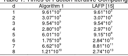
[image:8.595.192.399.413.504.2]

According to Algorithm 1, we assume that the number of node of each layer is 30, then we can obtain the time of iterative computation of all functions by computing. When the alternation depth

d

takes a different value, the number of iteration is as Table 1. Table 1 shows that our algorithm is more efficient.

Table 1. Times of Fuction Iterative Computing

d Algorithm 1 LAFP [15] 1 9.61*102

9.61*102

2 3.07*104

3.07*104

3 9.54*105 9.54*105 4 2.80*106 2.97*107 5 6.01*107

9.15*108

6 1.75*108

2.84*1010

7 6.62*109 8.81*1011 8 1.21*1010 2.74*1013

4. Conclusion

In this paper, we present a new efficient algorithm for evaluating PDG fixpoints. As we know, [26] presented a local model checker forμ-calculus, as a tableau system, but it did not analyze the computational complexity. Then [15] presented a new local algorithm for evaluating PDG fixpoints, and time complexity of the LAFP algorithm was exponential relationship with nesting depth. After a detailed analysis, we present a new algorithm by[11]. And our algorithm takes about

d n

2



d/2+2 steps. Clearly, the time required by our algori thm is only about the square root of the time required by LAFP algorithm. Furthermore, when

d

mod 2 1



, we only need to design the algorithm in the same way as

d

mod 2



0

. The nested bound algorithm reduces repetitive computation and improves the computational efficiency. The research in this paper is very important to theoretical research and practical application [25, 27], it can improve the efficiency for verifying hardware and software designs.

Acknowledgements

This paper is supported by the National Natural Science Foundation of China under Grant No.61472406, the Natural Science Foundation of Fujian Province under Grant No.2015J01269 and No.2016J01304 and the Talent Introduction Foundation of Minnan Normal University.

References

[1] D Kozen. Results on the propositional μ-calculus. LNCS 140: Proc of the 9th Colloquium on Automata, Languages and Programming. Springer. 1982: 348-359.

[2] JW de Bakker. Mathematical theory of program correctness. Prentice-Hall, Inc. 1980.

[3] D Park. Fixpoint induction and proof of program semantics. In: B Meltzer, D Michie. Editors. Mach. Int, Edinburgh Univ. 1970: 59-78.

[4] C Stirling. Modal and temporal logics for processes. Springer. 1996: 149-237.

[5] A Tarski. A lattice-theoretical fixpoint theorem and its applications. Pacific Journal of Mathematics.

1955; 5(2): 285-309.

[6] EA Emerson, CL Lei. Efficient model checking in fragments of the propositional mu-calculus. Proc. 1st LICS. 1986.

[7] HR Andersen. Model checking and boolean graphs. ESOP 92. Springer. 1992: 1-19.

[8] R Cleaveland, M Klein, B Steen. Faster model checking for the modal mu-calculus. CAV 92, LNCS. 1992; 663: 410-422.

[9] R Cleaveland. Tableau-based model checking in the prepositional mucalculus. Acta Informatica. 1990; 27(8): 725-747.

[10] DE Long, A Browne, EM Clarke, et al. An improved algorithm for the evaluation of fixpoint expressions. Computer Aided Verification. 1994: 338-350.

[11] H Jiang. Efficient global model-checking for propositional μ-calculus. Journal of Computer Research and Development. 2010; 47(8): 1424-1433.

[12] HR Andersen. Model checking and boolean graphs. Theoretical Computer Science. 1994; 126(1). [13] B Vergauwen, J Lewi. Efficient local correctness checking for single and alternating boolean equation

systems. Proceedings of ICALP 94. Springer. 1994: 304-315.

[14] GS Bhat, R Cleaveland. Efficient model checking for fragments of the modal μ-calculus. Proceedings of the Second International Workshop on Tools and Algorithms for the Construction and Analysis of Systems (TACAS 96). Springer. 1996: 107-126.

[15] XX Liu, CR Ramakrishnan, SA Smolka. Fully local and efficient evaluation of alternating fixed points.

Tools and Algorithms for the Construction and Analysis of Systems. 1998: 5-19.

[16] R Mateescu. Local model-checking of modal mu-calculus on acyclic labeled transition systems. Tools and Algorithm for the Construction and Analysis of Systems. 2002: 281-295.

[17] JF Jensen, LK Østergaard. Local model checking of weighted CTL. 2012.

[18] D Latella, M Loreti, M Massink. On-the-fly fast mean-field modelchecking. Trustworthy Global Computing. Springer International Publishing, LNCS. 2014: 297-314.

[19] R Guerraoui, M Yabandeh. Local model checking. 2011.

[20] JF Jensen, KG Larsen, J Srba, et al. Local model checking of weighted CTL with upper-bound constraints. Model Checking Software. 2013: 178-195.

[21] Hua Jiang, Jianqing Xi. Improved algorithm of golbal model-checking for propositional mu-calculus.

Applied Mechanics and Materials. 2013; 263: 2314-2319.

[22] Liu Wanwei, et al. A Simple Probabilistic Extension of Modal Mu-calculus. 2015.

[23] Castro Pablo, Cecilia Kilmurray, Nir Piterman. Tractable Probabilistic μ-Calculus that Expresses Probabilistic Temporal Logics. 2015.

[24] EM Clarke, O Grumberg, D Peled. Model checking. MIT Press. 1999.

[25] N Piterman, MY Vardi. Global model-checking of infinite-state systems. Computer Aided Verification.

2004: 387-400.

[26] C Stirling, D Walker. Local model checking in the modal mu-calculus. Theoretical Computer Science.

1991; 89(1): 161-177.