Linguistic Matrix Theory

(1)

QMUL-PH-17-03

Linguistic Matrix Theory

Dimitrios Kartsaklis

a,1

, Sanjaye Ramgoolam

b,c,2

, Mehrnoosh Sadrzadeh

a,3

a _{School of Electronic Engineering and Computer Science,}

Queen Mary University of London, Mile End Road,

London E1 4NS, UK

b _{Centre for Research in String Theory, School of Physics and Astronomy}_,

Queen Mary University of London,

Mile End Road, London E1 4NS, UK

c _{National Institute for Theoretical Physics,}

School of Physics and Centre for Theoretical Physics, University of the Witwatersrand, Wits, 2050, South Africa

ABSTRACT

Recent research in computational linguistics has developed algorithms which associate matrices with adjectives and verbs, based on the distribution of words in a corpus of text. These matrices are linear operators on a vector space of context words. They are used to construct the meaning of composite expressions from that of the elementary constituents, forming part of a compositional distributional approach to semantics. We propose a Matrix Theory approach to this data, based on permutation symmetry along with Gaussian weights and their perturbations. A simple Gaussian model is tested against word matrices created from a large corpus of text. We characterize the cubic and quartic departures from the model, which we propose, alongside the Gaussian parameters, as signatures for comparison of linguistic corpora. We propose that perturbed Gaussian models with permutation symmetry provide a promising framework for characterizing the nature of universality in the statistical properties of word matrices. The matrix theory framework developed here exploits the view of statistics as zero dimensional perturbative quantum field theory. It perceives language as a physical system realizing a universality class of matrix statistics characterized by permutation symmetry.

1

d.kartsaklis@qmul.ac.uk

2

s.ramgoolam@qmul.ac.uk

3

mehrnoosh.sadrzadeh@qmul.ac.uk

(2)

Introduction

(3)

similarity of words by application of vector algebra tools [3, 4], their statistical nature do not allow them to scale up to the level of multi-word phrases or sentences. Recent methods [5, 6, 7, 8, 9] address this problem by adopting a compositional approach: the meaning of relational words such as verbs and matrices is associated with matrices or higher order tensors, and composition with the noun vectors takes the form of tensor contraction. In tensor-based models of this form, the grammatical type of each word determines the vector space in which the word lives: takeN to be the noun space and S the sentence space, then an adjective becomes a linear mapN →N living inN∗_⊗_N_{, an} intransitive verb a map N → S in N∗ _⊗_{S, and a transitive verb a tensor of order 3 in} N∗_⊗_S_⊗_N∗_{. Hence, given a transitive sentence of the form “John likes Mary”, vectors}

−−−→

John,−−−→M aryrepresenting the meaning of the noun arguments and an order-3 tensorMlikes

for the verb, the meaning of the sentence is a vector in S computed as −−−→JohnMlikes

−−−→

M ary. Given this form of meaning representation, a natural question is how to characterize the distribution of the matrix entries for all the relational words in the corpus, which correspond to a vast amount of data. Our approach to this problem is informed by Random Matrix theory. Random matrix theory has a venerable history starting from Wigner and Dyson [10, 11] who used it to describe the distribution of energy levels of complex nuclei. A variety of physical data in diverse physical systems has been shown to obey random matrix statistics. The matrix models typically considered have continuous symmetry groups which relate the averages and dispersions of diagonal and off-diagonal elements of the matrix elements. Our study of these averages in the context of language shows that there are significant differences between these characteristics for diagonal and off-diagonal elements.

This observation motivates the study of a simple class of solvable Gaussian models without continuous symmetry groups. In the vector/tensor space models of language meaning, it is natural to expect a discrete symmetry of permutations of the context words used to define the various vectors and tensors. Random matrix integrals also arise in a variety of applications in theoretical physics, typically as the reductions to zero dimensions from path integrals of a higher dimensional quantum field theory. We develop a matrix theory approach to linguistic data, which draws on random matrix theory as well as quantum field theory, and where the permutation symmetry plays a central role.

The paper is organised as follows:

Section 2 gives some more detailed background on how random matrices arise in applied and theoretical physics, highlighting the role of invariant functions of matrix variables in the definition of the probability measure and the observables.

Section 3 describes the main ideas behind distributional models of meaning at the word level, and explains how the principle of compositionality can be used to lift this concept to the level of phrases and sentences.

(4)

about constructing vectors for nouns and matrices for verbs and adjectives by application of linear regression.

Section 5 presents data on distributions of several selected matrix elements which motivates us to consider Gaussian measures as a starting point for connectingSD invariant probability distributions with the data. Section 6 describes a 5-parameter Gaussian model. Section 7 discusses the comparison of the theory with data. Finally, Section 8 discusses future directions.

2

Random matrices: Observables and symmetries

The association of relational words such as adjectives and verbs in a corpus with matrices produces a large amount of matrix data, and raises the question of characterising the information present in this data. Matrix distributions have been studied in a variety of areas of applied and theoretical physics. Wigner and Dyson studied the energy levels of complex nuclei, which are eigenvalues of hermitian matrices. The techniques they developed have been applied to complex atoms, molecules, subsequently to scattering matrices, chaotic systems amd financial correlations. Some references which will give an overview of the theory and diversity of applications of random matrix theory are [12, 13, 14, 15]. The spectral studies of Wigner and Dyson focused on systems with continuous symmetries, described by unitary, orthogonal or symplectic groups.

Matrix theory has also seen a flurry of applications in fundamental physics, an impor-tant impetus coming from the AdS/CFT correspondence [16], which gives an equivalence between four dimensional quantum field theories and ten dimensional string theory. These QFTs have conformal invariance and quantum states correspond to polynomials in matrix fields M(~x, t), invariant under gauge symmetries, such as the unitary groups. Thanks to conformal invariance, important observables in the string theory are related to quantities which can be computed in reduced matrix models where the quantum field theory path integrals simplify to ordinary matrix integrals (for reviews of these directions in AdS/CFT see [17, 18]). This sets us back to the world of matrix distributions. These matrix inte-grals also featured in earlier versions of gauge-string duality for low-dimensional strings, where they find applications in the topology of moduli spaces of Riemann surfaces (see [19] for a review).

An archetypal object of study in these areas of applied and theoretical physics is the matrix integral

Z(M) =

Z

dM e−trM2 (2.1)

which defines a Gaussian Matrix distribution, and the associated matrix moments

Z

(5)

Moments generalizing the above are relevant to graviton interactions in ten-dimensional string theory in the context of AdS/CFT. Of relevance to the study of spectral data, these moments contain information equivalent to eigenvalue distributions, since the matrix measure can be transformed to a measure over eigenvalues using an appropriate Jacobian for the change of variables. More generally, perturbations of the Gaussian matrix measure are of interest:

Z(M, g) =

Z

dM e−trM2+PkgktrMk _(2.3)

for coupling constants gk. In the higher dimensional quantum field theories, the gk are coupling constants controlling the interaction strengths of particles.

In the linguistic matrix theory we develop here, we study the matrices coming from linguistic data using Gaussian distributions generalizing (2.1)-(2.3). The matrices we use are not hermitian or real symmetric; they are general real matrices. Hence, a distribution of eigenvalues is not the natural way to study their statistics. Another important property of the application at hand is that while it is natural to consider matrices of a fixed size D×D, there is no reason to expect the linguistic or statistical properties of these matrices to be invariant under a continuous symmetry. It is true that dot products of vectors (which are used in measuring word similarity in distributional semantics) are invariant under the continuous orthogonal groupO(D). However, in general we may expect no more than an invariance under the discrete symmetric groupSD ofD! permutations of the basis vectors. The general framework for our investigations will therefore be Gaussian matrix inte-grals of the form:

Z

dM eL(M)+Q(M)+perturbations _(2.4)

where L(M) is a linear function of the matrix M, invariant under SD, and Q(M) is a quadratic function invariant under SD. Allowing linear terms in the Gaussian action means that the matrix model can accommodate data which has non-zero expectation value. The quadratic terms are eleven in number forD≥4, but we will focus on a simple solvable subspace which involves three of these quadratic invariants along with two linear ones. Some neat SD representation theory behind the enumeration of these invariants is explained in Appendix B. The 5-parameter model is described in Section 6.

3

Vectors and tensors in linguistics: Theory

3.1

Distributional models of meaning

(6)

of a word is defined by the contexts in which it occurs [1, 2]. In a distributional model of meaning, a word is represented as a vector of co-occurrence statistics with a selected set of possible contexts, usually single words that occur in the same sentence with the target word or within a certain distance from it. The statistical information is extracted from a large corpus of text, such as the web. Models of this form have been proved quite successful in the past for evaluating the semantic similarity of two words by measuring (for example) the cosine distance between their vectors.

For a wordwand a set of contexts{c1, c2,· · · , cn}, we define the distributional vector

of w as:

−

→_w _{= (f}_(c

1), f(c2),· · · , f(cn)) (3.1)

where in the simplest case f(ci) is a number showing how many times w occurs in close proximity toci. In practice, the raw counts are usually smoothed by the application of an appropriate function such aspoint-wise mutual information (PMI). For a context wordc and a target word t, PMI is defined as:

P M I(c, t) = log p(c, t)

p(c)p(t) = log p(c|t)

p(c) = log p(t|c)

p(t) = log

count(c, t)·N

count(t)·count(c) (3.2) where N is the total number of tokens in the text corpus, and count(c, t) is the number of c and t occurring in the same context. The intuition behind PMI is that it provides a measure of how often two events (in our case, two words) occur together, with regard to how often they occur independently. Note that a negative PMI value implies that the two words co-occur less often that it is expected by chance; in practice, such indications have been found to be less reliable, and for this reason it is more common practice to use the positive version of PMI (often abbreviated as PPMI), in which all negative numbers are replaced by 0.

One problem with distributional semantics is that, being purely statistical in nature, it does not scale up to larger text constituents such as phrases and sentences: there is simply not enough data for this. The next section explains how theprinciple of compositionality

can be used to address this problem.

3.2

Grammar and tensor-based models of meaning

The starting point of tensor-based models of language is a formal analysis of the gram-matical structure of phrases and sentences. These are then combined with a semantic analysis, which assigns meaning representations to words and extends them to phrases and sentences compositionally, based on the grammatical analysis:

(7)

The grammatical structure of language has been made formal in different ways by different linguists. We have the work of Chomsky on generative grammars [20], the original functional systems of Ajdukiewicz [21] and Bar-Hillel [22] and their type logical reformulation by Lambek in [23]. There is a variety of systems that build on the work of Lambek, among which the Combinatorial Categorial Grammar (CCG) of Steedman [24] is the most widespread. These latter models employ ordered algebras, such as residuated monoids, elements of which are interpreted as function-argument structures. As we shall see in more detail below, they lend themselves well to a semantic theory in terms of vector and tensor algebras via the map-state duality:

Ordered Structures =⇒Vector and Tensor Spaces

There are a few choices around when it comes to which formal grammar to use as base. We discuss two possibilities: pregroup grammars and CCG. The contrast between the two lies in the fact that pregroup grammars have an underlying ordered structure and form a partial order compact closed category [25], which enables us to formalise the syntax-semantics passage as a strongly monoidal functor, since the category of finite dimensional vector spaces and linear maps is also compact closed (for details see [5, 26, 27]). So we have:

Pregroup Algebrasstrongly monoidal functor=⇒ Vector and Tensor Spaces

In contrast, CCG is based on a set of rules, motivated by the combinatorial calculus of Curry [28] that was developed for reasoning about functions in arithmetics and extended and altered for purposes of reasoning about natural language constructions. The CCG is more expressive than pregroup grammars: it covers the weakly context sensitive fragment of language [29], whereas pregroup grammars cover the context free fragment [30].

3.3

Pregroup grammars

A pregroup algebra (P,≤,·,1,(−)r_,₍₋₎l_{) is a partially ordered monoid where each element} p∈P has a left pl _{and right} _pr _{adjoint, satisfying the following inequalities:}

p·pr≤1≤pr·p pl·p≤1≤p·pl

A pregroup grammar over a set of words Σ and a set of basic grammatical types is denoted by (P(B),R)Σ where P(B) is a pregroup algebra generated over B and R is a relation

R ⊆ Σ× P(B) assigning to each word a set of grammatical types. This relation is otherwise known as alexicon. Pregroup grammars were introduced by Lambek [31], as a simplification of his original Syntactic Calculus [23].

(8)

pregroup grammar over Σ andB has the following lexicon:

(men, n),(cats, n),(tall, n·nl),(snore, nr·s),(love, nr·s·nl)

Given a string of wordsw1, w2,· · · , wn, its pregroup grammar derivation is the

follow-ing inequality, for (wi, ti) an element of the lexicon of P(B) and t ∈P(B): t1·t2· · · ·tn≤t

When the string is a sentence, thent =s. For example, the pregroup derivations for the the phrase “tall men” and sentences “cats snore” and “men love cats” are as follows:

(n·nl₎_·_n_≤_n_·_{1 =}_n n·(nr_·_s)_≤₁_·_s₌_s

n·(nr·s·nl)·n ≤1·s·1 =s

In this setting the partial order is read as grammatical reduction. For instance, the juxtaposition of types of the words of a grammatically formed sentence reduces to the types, and a grammatically formed noun phrase reduces to the type n.

3.4

Combinatorial Categorial Grammar

Combinatorial Categorial Grammar has a set of atomic and complex categories and a set of rules. Complex types are formed from atomic types by using two slash operators\and /; these are employed for function construction and implicitly encode the grammatical order of words in phrases and sentences.

Examples of atomic categories are the types of noun phrases n and sentences s. Ex-amples of complex categories are the types of adjectives and intransitive verbs, n/n and s\n, and the type of transitive verbs, (s\n)/n. The idea behind these assignments is that a word with a complex typeX\Y or X/Y is a function that takes an argument of the formY and returns a result of type X. For example, adjectives and intransitives verb are encoded as unary functions: an adjective such as “tall” takes a noun phrase of type n, such as “men” on its right and return a modified noun phrase n, i.e. “tall men”. On the other hand, an intransitive verb such as “snore” takes a noun phrase such as “cats” on its left and returns the sentence “cats snore”. A transitive verb, such as “loves” first takes an argument of typenon its right, e.g. “cat”, and produces a function of type s\n, for instance “love cats”, then takes an argument of type n on its left, e.g. “men” and produces a sentence, e.g. “men love cats”.

In order to combine words and form phrases and sentences, CCG employs a set of rules. The two rules which formalise the reasoning in the above examples are calledapplications

and are as follows:

(9)

tall men

n/n n =>⇒ n cats snore

n s\n =<⇒ s

men love cats

n (s\n)/n n =>⇒ n s\n =<⇒ n

3.5

Semantics

On the semantic side, we present material for the CCG types. There is a translation t between the CCG and pregroup types, recursively defined as follows:

t(X/Y) :=t(X)·t(Y)l t(X\Y) := t(Y)r·t(X)

This will enable us to use this semantics for pregroups as well. For a detailed semantic development based on pregroups, see [5, 26].

We assign vector and tensor spaces to each type and assign the elements of these spaces to the words of that type. Atomic types are assigned atomic vector spaces (tensor order 1), complex types are assigned tensor spaces with rank equal to the number of slashes of the type.

Concretely, to an atomic type, we assign a finite atomic vector space U; to a complex typeX/Y orX\Y, we assign the tensor spaceU⊗U. This is a formalisation of the fact that in vector spaces linear maps are, by the map-state duality, in correspondence with elements of tensor spaces. So, a noun such as “men” will get assigned a vector in the space U, whereas an adjective such as “tall” gets assigned a matrix, that is a linear map from U to U. Using the fact that in finite dimensional spaces choosing an orthonormal basis identifies U∗ _and _U_{, this map is an element of} _U _⊗_{U. Similarly, to an intransitive verb} “snores” we assign a matrix: an element of the tensor space U ⊗U, and to a transitive verb “loves”, we assign a “cube”: an element of the tensor spaceU ⊗U ⊗U.4

The rules of CCG are encoded as tensor contraction. In general, for Tij···z an element of X⊗Y ⊗ · · · ⊗Z and Vj an element of Z, we have that:

Tij···zVz

In particular, given an adjectiveAdjij ∈U⊗U and a nounVj ∈U, the corresponding noun vectorAdjijVj, e.g. “tall men” istallijmenj. Similarly, an intransitive verbItvij ∈U⊗U is applied to a noun Vj ∈ U and forms the sentence ItvijVj, e.g. for “mens snore” we obtain the vector snoreijmenj. Finally, a transitive verb T vijk ∈ U ⊗U ⊗U applies to nouns Wj, Vk ∈ U and forms a transitive sentence (V rbijkVk)Wj, e.g. “cats chase mice” corresponds the vector (chaseijkmicek)catsj.

4

(10)

Given this theory, one needs to concretely implement the vector space U and build vectors and tensors for words. The literature contains a variety of methods, ranging from analytic ones that combine arguments of tensors [6, 9, 32, 33], linear and multi linear regression methods [8, 34, 35], and neural networks [7]. The former methods are quite specific; they employ assumptions about their underlying spaces that makes them unsuit-able for the general setting of random matrix theory. The neural networks methods used for building tensors are a relatively new development and not widely tested in practice. In the next section, we will thus go through the linear regression method described in [8, 34], which is considered a standard approach for similar tasks.

4

Vectors and tensors in linguistics: Practice

Creating vectors and tensors representing the meaning of words requires a text corpus sufficiently large to provide reliable statistical knowledge. For this work, we use a con-catenation of the ukWaC corpus (an aggregation of texts from web pages extracted from the .uk domain) and a 2009 dump of the English Wikipedia5_{—a total of 2.8 billion tokens}

(140 million sentences). The following sections detail how this resource has been used for the purposes of the experimental work presented in this paper.

4.1

Preparing a dataset

We work on the two most common classes of content words with relational nature: verbs and adjectives. Our study is based on a representative subset of these classes extracted from the training corpus, since the process of creating matrices and tensors is compu-tationally expensive and impractical to be applied on the totality of these words. The process of creating the dataset is detailed below:

1. We initially select all adjectives/verbs that occur at least 1000 times in the corpus, sort them by frequency, and discard the top 100 entries (since these aretoofrequent, occurring in almost every context, so less useful for the purpose of this study). This produces a list of 6503 adjectives and 4385 verbs.

2. For each one of these words, we create a list of arguments: these are nouns modified by the adjectives in the corpus, and nouns occurring as objects for the verb case. Any argument that occurs less than 100 times with the specific adjective/verb is discarded as non-representative.

3. We keep only adjectives and verbs that have at least 100 arguments according to the selection process of Step 2. This produced a set of 273 adjectives and 171 5

(11)

verbs, which we use for the statistical analysis of this work. The dataset is given in Appendix C.

The process is designed to put emphasis on selecting relational words (verbs/adjectives) with a sufficient number of relatively frequent noun arguments in the corpus, since this is very important for creating reliable matrices representing their meaning, a process described in Section 4.3.

4.2

Creating vectors for nouns

The first step is the creation of distributional vectors for the nouns in the text corpus, which grammatically correspond to atomic entities of language, and will later form the raw material for producing the matrices of words with relational nature, i.e. verbs and adjectives. The basis of the noun vectors consists of the 2000 most frequentcontentwords in the corpus,6 _{that is, nouns, verbs, adjectives, and adverbs. The elements of the vector}

for a wordwreflect co-occurrence counts ofwwith each one the basis words, collected from the immediate context ofw(a 5-word window from either side of w), for each occurrence of w in the training corpus. As it is common practice in distributional semantics, the raw counts have been smoothed by applying positive PMI (Equation 3.2). Based on this method, we create vectors for all nouns occurring as arguments of verbs/adjectives in our dataset.

4.3

Creating matrices for verb and adjectives

Our goal is to use the noun vectors described in Section 4.2 in order to create appro-priate matrices representing the meaning of the verbs and adjectives in a compositional

setting. For example, given an adjective-noun compound such as “red car”, our goal is to produce a matrix Mred such that Mred−→car=−→y, where −→car is the distributional vector of “car” and −→y a vector reflecting the distributional behaviour of the compound “red car”. Note that a non-compositional solution for creating such a vector −→y would be to treat the compound “red car” as a single word and apply the same process we used for creating the vectors of nouns above [8, 34]. This would allow us to create a dataset of the form {(−→car,−−−−→red car),(−−→door,−−−−−→red door),· · · } based on all the argument nouns of the specific adjective (or verb for that matter); the problem of finding a matrix which, when contracted by the vector of a noun, will approximate the distributional vector of the whole compound, can be solved by applying multi-linear regression on this dataset.7

Take matrices X and Y, where the rows ofX correspond to vectors of the nouns that occur as arguments of the adjective, and the rows of Y to the distributional vectors of

6

Or subsets of the 2000 most frequent content words for lower dimensionalities.

7

(12)

the corresponding adjective-noun compounds. We would like to find a matrix M that minimizes the distance of the predicted vectors from the actual vectors (the so-called

least-squares error), expressed in the following quantity: 1

2m ||M X T

−YT||2+λ||M||2

(4.1) where m is the number of arguments, and λ a regularization parameter that helps in avoidingoverfitting: the phenomenon in which the model memorizes perfectly the training data, but performs poorly on unseen cases. This is an optimization problem that can be solved by applying an iterative process such as gradient descent, or even analytically, by computing M as below:

M = (XTX)−1XTY (4.2)

In this work, we use gradient descent in order to produce matrices for all verbs and adjectives in our dataset, based on their argument nouns. For each word we createD×D matrices for variousDs, ranging from 300 to 2000 dimensions in steps of 100; the different dimensionalities will be used later in Section 7 which deals with the data analysis. The selection procedure described in Section 4.1 guarantees that the argument set for each verb/adjective will be of sufficient quantity and quality to result in a reliable matrix representation for the target word.

It is worth noting that the elements of a verb or adjective matrix created with the linear regression method do not directly correspond to some form of co-occurrence statistics related to the specific word; the matrix acts as a linear map transforming the input noun vector to a distributional vector for the compound. Hence, the “meaning” of verbs and adjectives in this case is not directly distributional, but transformational, along the premises of the theory presented in Section 3.5.

5

Permutation symmetric Gaussian matrix models

Gaussian matrix models rely on the assumption that matrix elements follow Gaussian distributions. In the simplest models, such as the one in (2.2), we have equal means and dispersions for the diagonal and off-diagonal matrix elements. In the past, analytic calculations have been applied to obtain eigenvalue distributions, which were compared with data. In this work we take a different approach: a blend between statistics and effective quantum field theory guided by symmetries.

(13)

[image:13.612.103.502.93.389.2]

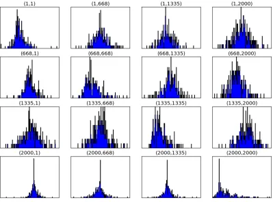
Figure 1: Histograms for elements of adjective matrices

reflects frequency (i.e. for how many words the specific element falls within the interval represented by the bar). These histograms, presented here for demonstrative purposes, look qualitatively like Gaussians.

This motivates an investigation of Gaussian statistics for word matrices, along the lines of random matrix theory. In the simplest physical applications, the means and variances of diagonal and off diagonal elements are equal for reasons related to underlying contin-uous symmetries. When M is a hermitian operator corresponding to the Hamiltonian of a quantum system described by states in a Hilbert space, there is a unitary symmetry preserving the inner product. Invariants under unitary group symmetries in this case are traces. The quadratic invariant trM2 _{sums diagonal and off-diagonal elements with}

(14)

elements in the unitary groupU(D). One can even imagine breaking the symmetry fur-ther by choosing the context words to be ordered according to their own frequency in the corpus. We do not make such special choices in our experiments. This gives very good motivation to consider the universality class of permutation symmetric models, based on the application to distributional models of meaning we are developing. As far as we are aware, such models have not been systematically studied in physics applications. Of course the framework of SD invariant models includes the more restricted models with larger symmetry at special values of the parameters.

The initial inspection of histograms for individual matrix elements provides a strong argument in favour of considering Gaussian matrix models in the linguistic context. A theoretical argument can be sought from the central limit theorem, which gives general mechanisms for Gaussian random variables to arise as the sums of other variables with finite mean and norm. A possible objection to this is that slowly decaying power laws with infinite variance are typical in linguistics, with Zipf’s law8 _{to be the most prominent}

amongst them. It has been shown, however, that Zipfian power laws in linguistics arise from more fundamental distributions with rapid exponential decay [37]. So there is hope for Gaussian and near-Gaussian distributions for adjectives and verbs to be derived from first principles. We will not pursue this direction here, and instead proceed to develop concrete permutation invariant Gaussian models which we compare with the data.

It is worth noting that, while much work on applications of matrix theory to data in physics focuses on eigenvalue distributions, there are several reasons why this is not the ideal approach here. The matrices corresponding to adjectives or intransitive verbs created by linear regression are real and not necessarily symmetric (M is not equal to its transpose); hence, their eigenvalues are not necessarily real.9 _{One could contemplate}

a Jordan block decomposition, where in addition to the fact that the eigenvalues can be complex, one has to keep in mind that additional information about the matrix is present in the sizes of the Jordan block. More crucially, since our approach is guided by SD symmetry, we need to keep in mind that general base changes required to bring a matrix into Jordan normal form are not necessarily in SD. The natural approach we are taking consists in considering all possibleSD invariant polynomial functions of the matrix M, and the averages of these functions constructed in a probability distribution which is itself function of appropriate invariants. Specifically, in this paper we will consider the probability distribution to be a simple 5-parameter Gaussian, with a view to cubic and quartic perturbations thereof, and we will test the viability of this model by comparing

8

Zipf’s law [36] is empirical and states that the frequency of any word in a corpus of text is inversely proportional to the rank of the word in the frequency table. This roughly holds for any text, for example it describes the distribution of the words in this paper.

9

(15)

to the data.

Perturbed Gaussian matrix statistics can be viewed as the zero dimensional reduction of four dimensional quantum field theory, which is used to describe particle physics, e.g. the standard model. The approach to the data we describe in more detail in the next section is the zero dimensional analog of using effective quantum field theory to describe particle physics phenomena, where symmetry (in the present caseSD) plays an important role.

6

The 5-parameter Gaussian model

We consider a simpleSD invariant Gaussian matrix model. The measuredM is a standard measure on the D2 matrix variables given in Section A.4. This is multiplied by an expo-nential of a quadratic function of the matrices. The parameters J0_{, J}S _{are coefficients of} terms linear in the diagonal and off-diagonal matrix elements respectively. The parameter Λ is the coefficient of the square of the diagonal elements, while a, b are coefficients for off-diagonal elements. The partition function of the model is

Z(Λ, a, b, J0, JS) =

Z

dM e−Λ2

PD i=1Mii2−

1 4(a+b)

P

i<j(Mij2+Mji2)

e−12(a−b)

P

i<jMijMji+J0PiMii+JSPi<j(Mij+Mji) _(6.1)

The observables of the model are SD invariant polynomials in the matrix variables: f(Mi,j) =f(Mσ(i),σ(j)) (6.2)

At quadratic order there are 11 polynomials, which are listed in Section B.1. We have only used three of these invariants in the model above. The most general matrix model compatible withSD symmetry would consider all the eleven parameters and allow coefficients for each of them. In this paper, we restrict attention to the simple 5-parameter model, where the integral factorizes intoDintegrals for the diagonal matrix elements and D(D−1)/2 integrals for the off-diagonal elements. Each integral for a diagonal element is a 1-variable integral. For each (i, j) with i < j, we have an integral over 2 variables.

Expectation values of f(M) are computed as

hf(M)i ≡ 1 Z

Z

dM f(M)EXP (6.3)

(16)

equation (A.10). Taking appropriate derivatives of the result gives the expectation values of the observables.

Since the theory is Gaussian, all the correlators can be given by Wick’s theorem in terms of the linear and quadratic expectation values, as below:

hMiji = 2J S

a for all i6=j

hMiii = Λ−1J0 (6.4)

For quadratic averages we have:

hMiiMjji = hMiiihMjji + δijΛ−1

hMijMkli = hMijihMkli+ (a−1+b−1)δikδjl+ (a−1 −b−1)δilδjk (6.5) From the above it also follows that:

hMiiMjjic = δijΛ−1

hMijMijic = (a−1+b−1) for i6=j

hMijMjiic = (a−1−b−1) for i6=j (6.6)

6.1

Theoretical results for

S

D

invariant observables

In this section we give the results for expectation values of observables, which we will need for comparison to the experimental data, i.e. to averages over the collection of word matrices in the dataset described in Section 4.1. The comparison of the linear and quadratic averages are used to fix the parameters J0, JS,Λ, a, b. These parameters are

then used to give the theoretical prediction for the higher order expectation values, which are compared with the experiment.

6.1.1 Linear order

Md:1=

* X

i Mii

+

=htrMi= Λ−1J0D

Mo:1 =

* X

i6=j Mij

+

= 2D(D−1) a J

S

(17)

6.1.2 Quadratic order

Md:2 =

X

i

hMii2i=

X

i

hMiiihMiii+X i

Λ−1 =DΛ−2(J0)2 +DΛ−1 Mo:2,1 =

X

i6=j

hMijMiji=X i6=j

hMijihMiji+X i6=j

(a−1+b−1) =D(D−1) 4(JS)2a−2+ (a−1+b−1)

Mo:2,2 =

X

i6=j

hMijMjii=D(D−1) 4(JS)2a−2+ (a−1−b−1)

(6.8)

6.1.3 Cubic order

Md:3 ≡

X

i

hM3

iii=

X

i

hMiii3_{+ 3}X

i

hM2

iiic hMiii =DΛ−3(J0)3+ 3DΛ−2(J0) Mo:3,1 ≡

X

i6=j

hM3

iji=

X

i6=j

hMiji3_{+ 3}X

i6=j

hMijMijichMiji

=D(D−1)

(2Js a )

3₊6Js

a (a

−1₊_b−1₎

Mo:3,2 =

X

i6=j6=k

hMijMjkMkii= 8D(D−1)(D−2)(JS)3a−3 (6.9)

6.1.4 Quartic order

Md:4 =

X

i

hM_ii4i=DΛ−2

Λ−2(J0)4+ 6Λ−1(J0)2+ 3

Mo;4,1 =

X

i6=j

hMij4i=

X

i6=j

hMiji4+ 6hMijMijichMiji2+ 3hMijMiji2c

=D(D−1)

2Js a 4 + 6 2Js a 2

(a−1 +b−1) + 3(a−1+b−1)2

!

Mo:4,2 =

X

i6=j6=k6=l

hMijMjkMklMlii= 16D(D−1)(D−2)(D−3)a−4(JS)4

(18)

7

Comparison of Gaussian models and linguistic data

An ideal theoretical model would be defined by a partition function

Z(M) =

Z

dM e−S(M) (7.1)

with some appropriate functionS(M) (the Euclidean action of a zero dimensional matrix quantum field theory) such that theoretical averages

hf(M)i= 1

Z

dM e−S(M)_f(M₎ _(7.2)

would agree with experimental averages

hf(M)iEXP T =

1

Number of words

X

words

fword(M) (7.3)

to within the intrinsic uncertainties in the data, due to limitations such as the small size of the dataset.

In the present investigation we are comparing a Gaussian theory with the data, which is well motivated by the plots shown earlier in Figure 1. The differences between theory and experiment can be used to correct the Gaussian theory, by adding cubic and quartic terms (possibly higher) to get better approximations to the data. This is in line with how physicists approach elementary particle physics, where the zero dimensional matrix inte-grals are replaced by higher dimensional path inteinte-grals involving matrices, the quadratic terms in the action encode the particle content of the theory, and higher order terms encode small interactions in perturbative quantum field theory: a framework which works well for the standard model of particle physics.

We use the data for the averages Md:1, Mo:1 , Md:2 , Mo:2,1, and Mo:2,2 to determine

the parametersJ0,Λ, Js, a, b of the Gaussian Matrix model for a range of values of D(the

number of context words) ranging from D= 300 to D= 2000, increasing in steps of 100. Working with the adjective part of the dataset, we find:

J0

D = 1.31×10 −2

Λ

D2 = 2.86×10

−3

Js

D = 4.51×10 −4

a

D2 = 1.95×10

−3

b

D2 = 2.01×10

(19)

[image:19.612.180.408.91.237.2]

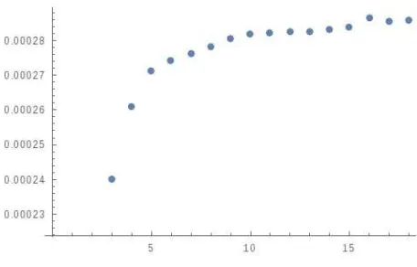
Figure 2: The ratio _DΛ2 stabilzing at largeD.

The plot in Figure 2 shows that the ratio _DΛ2 approaches a constant as D increases towards large values. Plots for the other ratios above show a similar stabilization. The calculation of the averages were repeated by permuting the set of 2000 context words, and repeating the calculation for different values ofD. In these two experiments, the values of the parameters at an intermediateD around 1200 are compared. The two sets of context words only have a partial overlap, due to the fact that both come from the same 2000 contexts. We find differences in the parameters of order one percent. We thus estimate that the random choice of context words results in an uncertainty of this order.

Using these Gaussian parameters, we can calculate the expectation values of a number of cubic and quartic invariants in the matrix model, which we then compare with the experimental values. The difference between diagonal cubic correlators in theory and experiment is small. We have:

(MdTHRY:3 /MdEXPT:3 ) = 0.57 (7.5)

indicating a percentage difference of 43%. As a next step in the theory/experiment com-parison, we would contemplate adding cubic terms to the Gaussian exponentials, following the philosophy of perturbative quantum field theory, adapted here to matrix statistics. We would then use these peturbations to obtain better estimates of cubic and higher order averages. The difference of 0.43 can be used as a sensible estimate of the size of the perturbation parameter. Calculations of up to fifth order would then reach accuracies of around one percent, comparable to the one percent uncertainties discussed above. This is a reasonable order of perturbative calculation comparable to what can be achieved in perturbative quantum field theory. The latter involves substantial additional complexity due to integrals over four-dimensional space-time momenta.

(20)

where universal features are likely to be manifest. For the quartic diagonal average we have:

(MdTHRY:4 /MdEXPT:4 ) = 0.33 (7.6)

with a percentage difference of 0.67. While the data is again not Gaussian at the level of reliability, this is still a very realistic set-up for perturbation theory around the Gaussian model.

For the simplest off-diagonal moments, the difference between experiment and theory is larger, but still within the realm of perturbation theory:

(M_oTHRY_:3_,₁ /M_oEXPT_:3_,₁ ) = 0.32

(MoTHRY:4,1 /MoEXPT:4,1 ) = 0.47 (7.7)

However, once we move to the more complex off-diagonal moments involving triple sums, the differences between theory and experiment start to become very substantial:

(M_oTHRY_:3_,₂ /M_oEXPT_:3_,₂ ) = 0.013

(MoTHRY:4,2 /MoEXPT:4,2 ) = 0.0084 (7.8)

In the framework of permutation symmetric Gaussian models we are advocating, this is in fact not surprising. As already mentioned, the 5-parameter Gaussian Matrix model we have considered is not the most general allowed by the symmetries. There are other quadratic terms we can insert into the exponent, for example:

e−cPi6=j6=kMijMjk _(7.9)

for some constant. This will lead to non-zero two-point averages:

hMijMjki − hMijihMjki (7.10) By considering c as a perturbation around the 5-parameter model in a limit of small c, we see that this will affect the theoretical calculation for

X

i6=j6=k

hMijMjkMkii (7.11)

A similar discussion holds for the matrix statistics for the verb part of the dataset. The parameters of the Gaussian model are now:

J0

D = 1.16×10 −3

Λ

D2 = 2.42×10

(21)

Js

D = 3.19×10 −4

a

D2 = 1.58×10

−3

b

D2 = 1.62×10

−3 _(7.12)

The cubic and quartic averages involving two sums over D show departures from Gaussianity which are broadly within reach of a realistic peturbation theory approach:

(MTHRY

d:3 /MdEXPT:3 ) = 0.54

(MdTHRY:4 /MdEXPT:4 ) = 0.30

(MoTHRY:3,1 /MoEXPT:3,1 ) = 0.25

(MoTHRY:4,1 /MoEXPT:4,1 ) = 0.48 (7.13)

The more complex cubic and quartic averages show much more siginificant differences between experiment and theory, which indicates that a more general Gaussian should be the starting point of perturbation theory:

(MoTHRY:3,2 /MoEXPT:3,2 ) = 0.010

(MoTHRY:4,2 /MoEXPT:4,2 ) = 0.006 (7.14)

The most general quadratic terms compatible with invariance under SD symmetry are listed in the Appendix B. While there are eleven of them, only three were included (along with the two linear terms) in the 5-parameter model. Taking into account some of the additional quadratic terms in the exponential of (6.1) will require a more complex theretical calculation in order to arrive at the predictions of the theory. While the 5-parameter integral can be factored into a product of integrals for each diagonal matrix element and a product over pairs{(i, j) :i < j}, this is no longer the case with the more general Gaussian models. It will require the diagonalization of a more complex bilinear form coupling the D2 _variables_Mij_.

In the Appendix B we also discuss higher order invariants of general degree k using representation theory ofSD and observe that these invariants are in correspondence with directed graphs. From a data-analysis perspective, the averages over a collection of word matrices of these invariants form the complete set of characteristics of the specific dataset. From the point of view of matrix theory, the goal is to find an appropriate weight of the form “Gaussian plus peturbations” which will provide an agreement with all the observable averages to within uncertainties intrinsic to the data.

(22)

gives a matrix theory. The fact that the standard model of particle physics is renormaliz-able means that the reduced matrix statistics of gluons and other particles involves only low order perturbations of Gaussian terms. It would be fascinating if language displays analogs of this renormalizability property.

8

Discussion and future directions

We find evidence that perturbed Gaussian models based on permutation invariants pro-vide a viable approach to analyzing matrix data in tensor-based models of meaning. Our approach has been informed by matrix theory and analogies to particle physics. The broader lesson is that viewing language as a physical system and characterizing the univer-sality classes of the statistics in compositional distributional models can provide valuable insights. In this work we analyzed the matrix data of words in terms of permutation symmetric Gaussian Matrix models. In such models, the continuous symmetries SO(D), Sp(D),U(D) typically encountered in physical systems involving matrices of sizeD, have been replaced by the symmetric groups SD. The simplest 5-parameter Gaussian models compatible with this symmetry were fitted to 5 averages of linear and quadratic SD in-variants constructed from the word matrices. The resulting model was used to predict averages of a number of cubic and quartic invariants. Some of these averages were well within the realm of perturbation theory around Gaussians. However, others showed sig-nificant departures which motivates a more general study of Gaussian models and their comparison with linguistic data for the future. The present investigations have established a framework for this study which makes possible a number of interesting theoretical as well as data-analysis projects suggested by this work.

An important contribution of this work is that it allows the characterization of any text corpus or word class in terms of thirteen Gaussian parameters: the averages of two linear and eleven quadratic matrix invariants listed in Appendix B. This can potentially provide a useful tool that facilitates research on comparing and analyzing the differences between:

• natural languages (e.g. English versus French)

• literature genres (e.g. The Bible versus The Coran; Dostoyevski versus Poe; science fiction versus horror)

• classes of words (e.g. verbs versus adjectives)

(23)

address data sparsity problems and lead to more robust distributional representations of meaning.

Furthermore, while we have focused on matrices, in general higher tensors are also involved (for example, a ditransitive verb10 is a tensor of order 4). The theory of per-mutation invariant Gaussian matrix models can be extended to such tensors as well. For the case of continuous symmetry, the generalization to tensors has been fruitfully studied [39] and continues to be an active subject of research in mathematics. Algebraic tech-niques for the enumeration and computation of corelators of tensor invariants [40] in the continuous symmetry models should continue to be applicable to SD invariant systems. These techniques rely on discrete dual symmetries, e.g. when the problem has manifest unitary group symmetries acting on the indices of one-matrix or multi-matrix systems, permutation symmetries arising from Schur-Weyl duality play a role. This is reviewed in the context of the AdS/CFT duality in [41]. When the manifest symmetry isSD, the symmetries arising from Schur-Weyl duality will involve partition algebras [42, 43].

As a last note, we would like to emphasize that while this paper draws insights from physics for analysing natural language, this analogy can also work the other way around. Matrix models are dimensional reductions of higher dimensional quantum field theories, describing elementary particle physics, which contain matrix quantum fields. In many cases, these models capture important features of the QFTs: e.g. in free conformal limits of quantum field theories, they capture the 2- and 3-point functions. An active area of research in theoretical physics seeks to explore the information theoretic content of quantum field theories [44, 45]. It is reasonable to expect that the application of the common mathematical framework of matrix theories to language and particle physics will suggest many interesting analogies, for example, potentially leading to new ways to explore complexity in QFTs by developing analogs of linguistic complexity.

Acknowledgments

The research of SR is supported by the STFC Grant ST/P000754/1, String Theory, Gauge Theory, and Duality; and by a Visiting Professorship at the University of the Wit-watersrand, funded by a Simons Foundation grant awarded to the Mandelstam Institute for Theoretical Physics. DK and MS gratefully acknowledge support by AFOSR Interna-tional Scientific Collaboration Grant FA9550-14-1-0079. MS is also supported by EPSRC for Career Acceleration Fellowship EP/J002607/1. We are grateful for discussions to An-dreas Brandhuber, Robert de Mello Koch, Yang Hao, Aurelie Herbelot, Hally Ingram, Andrew Lewis-Pye, Shahn Majid and Gabriele Travaglini.

10

(24)

A

Gaussian Matrix Integrals: 5-parameter model

M is a real D×D matrix. S and A are the symmetric and anti-symmetric parts. S= M +M

T 2 A= M−M

T

2 (A.1)

Equivalently,

Sij = 1

2(Mij+Mji) Aij = 1

2(Mij −Mji) (A.2)

We have:

ST =S AT =−A

M =S+A (A.3)

The independent elements of S are Sij for i≤ j, i.e the elements along the diagonal Sii and the elements above Sij for i < j. The independent elements of A are Aij for i < j. The diagonal elements are zero. Define:

dM = D

Y

i=1

dSiiY i<j

dSijdAij (A.4)

We consider the Gaussian partition function Z(Λ, B;J) =

Z

dM e−Pi

Λ_i 2 Mii−12

P

i<j(Sij,Aij)Bij(Sij,Aij)T _ePiJiiMii+Pi6=jJijMij _(A.5)

HereBij is a two by two matrix with positive determinant:

Bij =

aij cij cij bij

det(Bij) = aijbij −c2ij >0 (A.6) It defines the quadratic terms involving (Aij, Bij).

(Sij, Aij)Bij(Sij, Aij)T ₌_aij_S2

ij +bijA

2

(25)

is permutation symmetric. For simplicity, we will also choose c = 0. The linear terms (also called source terms) can be re-written as:

ePi6=jJijMij+PiJiMii ₌_ePiJiiMii+Pi<j(2JijSSij+2JijAAij) _(A.8)

whereJS

ij, JijA are the symmetric and anti-symmetric parts of the source matrix. JijS =

1

2(Jij +Jji) JA

ij = 1

2(Jij −Jji) (A.9)

Using a standard formula for multi-variable Gaussian integrals (see for example [46]):

Z(Λ, B;J) =

s

(2π)N2

Q

iΛi

Q

i<jdetBij e

1 2

P

iJiiΛ−i1Jii+Pi<j

2

det_Bij(bij(J

S

ij)2+aij(JijA)2−2cijJijAJijS)

(A.10) For any function of the matrices f(M) the expectation value is defined by:

hf(M)i= 1

Z

dM f(M) EXP (A.11)

where EXP is the product of exponentials defining the Gaussian measure. Following stan-dard techniques from the path integral approach to quantum field theory, the expectation values are calculated using derivatives with respect to sources (see e.g. [47]).

B

Counting

S

D

invariant matrix polynomials

There are 11 quadratic invariants in Mij which are invariant under SD ( D≥4).

X

i M_ii2

X

i6=j

M_ij2 , X i6=j

MijMji

X

i6=j

MiiMjj , X i6=j

MiiMij , X i6=j

MijMjj

X

i6=j6=k

MijMjk, X i6=j6=k

MijMik, X i6=j6=k

MijMkj, X i6=j6=k

MijMkk

X

i6=j6=k6=l

MijMkl (B.1)

(26)

P

i M2

ii

P

i6=j M2

ij

P

i6=j

MijMji P

i6=j

MiiMjj P

i6=j

MiiMij P

i6=j

MijMjj

P

i6=j6=k

MijMjkMki P

i6=j6=k

MijMik P

i6=j6=k

MijMkj P

i6=j6=k

MijMkk

P

i6=j6=k6=l

[image:26.612.87.507.98.315.2]

MijMkl

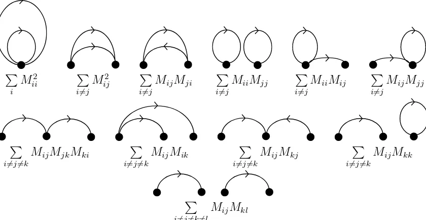
Figure 3: SD invariant functions and graphs illustrated for quadratic invariants

a directed edge connecting vertex i to vertex j, the above list corresponds to counting graphs. This connection between directed graphs and invariants is illustrated in Figure 3.

There is a representation theoretic way to obtain the counting formula as a function of the degreekof invariants (equal to 2 above) and the dimensionD. In our simple Gaussian theoretical model we have two linear terms along with the 3 quadratic terms in the first two lines of (B.1). A general Gaussian theory compatible with SD symmetry would take into account all the invariants. There are two linear invariants which can be averaged over the words. The experimental input into the Gaussian model would consist of the averages for all the invariants. Thus permutation symmetry leads to the characterization of matrices in tensor-based models of meaning by means of 13 Gaussian parameters. From a purely experimental point of view, it is interesting to also characterize the matrix data using further higher order invariants. Below, we explain the representation theory approach to the counting of higher order invariants.

LetVD be the D-dimensional permutation representation, also called the natural rep-resentation, of SD. The counting of invariants of degree k is the same as counting of 1-dimensional representations of SD in the decomposition into irreducibles of

Symk_(VD _⊗_VD₎ _(B.2)

This can be expressed in terms of characters. Define:

(27)

Given the linear forσ inVD which we denote as LD(σ), the linear operator inVD;2 is

LD;2(σ) = LD(σ)⊗ LD(σ) (B.4)

The tensor productVD⊗k;2 has an action ofσ as

LD;2;k(σ) = LD;2(σ)⊗ · · · ⊗ LD;2(σ) (B.5)

where we are takingk factors. The symmetric subspace of V_D⊗k_;2 is obtained by an action of permutationsτ ∈Sk, which involves permutating the k tensor factors. The dimension of this subspace is:

Dim(D, k) = 1 k!D!

X

σ∈SD

X

τ∈Sk

tr_V⊗k

D;2(LD;2;k(σ)τ)

= 1 D!k! X σ∈SD X τ∈Sk k Y i=1

(trVD;2(σ i

))Ci(τ) _(B.6)

Now use the fact that:

trVD;2(LD;2(σ)) = (trVD(LD(σ))

2 _{= (C}

1(σ))2 (B.7)

The last step is based on the observation that the trace of a permutation in the natural representation is equal to the number of one-cycles in the permutation. We also need:

trVD(LD(σ

i_{)) =}X

l|i

lCl(σ) (B.8)

This is a sum over divisors of i. We conclude:

Dim(D, k) = 1 D!k! X σ∈SD X τ∈Sk k Y i=1 (X l|i

lCl(σ))2Ci(τ) _(B.9)

The expression above is a function of the conjugacy classes of the permutations σ, τ. These conjugacy classes are partitions of D, k respectively, which we will denote by p=

{p1, p2,· · · , pD} and q ={q1, q2,· · · , qD} obeying Piipi =D,

P

iiqi =k. Thus

Dim(D, k) = 1 D!k! X p⊢D X q⊢k D! QD

i=1ipipi!

k!

Qk

i=1iqiqi!

k Y i=1   X l|i lpl  

2qi

(B.10)

(28)

matrix invariants. Hence the simplest formula for the number of invariants as a function of k is

Dim(2k, k) = X p⊢2k

X

q⊢k

1

Q

i=1ipi+qipi!qi!

k

Y

i=1

 

X

l|i lpl

 

2qi

(B.11)

Doing this sum in Mathematica, we find that the number of invariant functions at k = 2,3,4,5,6 are 11,52,296,1724,11060. These are recognized as the first few terms in the OEIS series A052171 which counts graphs (multi-graphs with loops on any number of nodes). The graph theory interpretatation follows by thinking aboutMij as an edge of a graph.

The decomposition ofV_D⊗k, and the closely related problem V_H⊗k whereVH is the non-trivial irrep of dimensionD−1 inVD, have been studied in recent mathematics literature [48] and are related to Stirling numbers. Some aspects of these decomposition numbers were studied and applied to the construction of supersymmetric states in quantum field theory [49].

C

Dataset

Below we provide the list of the 273 adjectives and 171 verbs for which matrices were constructed by linear regression, as explained in Section 4.3.

C.1

Adjectives

1st, 2nd, actual, adequate, administrative, adult, advanced, African, agricultural, alternative, amazing, ancient, animal, attractive, audio, Australian, automatic,

(29)

minute, mixed, mobile, model, monthly, moral, multiple, musical, Muslim, name, narrow, native, near, nearby, negative, net, nice, north, northern, notable, nuclear, numerous, official, ongoing, operational, ordinary, organic, outdoor, outstanding, overall, overseas, part, patient, perfect, permanent, Polish, positive, potential, powerful,

principal, prominent, proper, quality, quick, rapid, rare, reasonable, record, red, related, relative, religious, remote, residential, retail, rich, Roman, royal, rural, Russian, safe, scientific, Scottish, secondary, secret, selected, senior, separate, serious, severe, sexual, site, slow, soft, solid, sound, south, southern, soviet, Spanish, specialist, specified, spiritual, statutory, strange, strategic, structural, subsequent, substantial, sufficient, suitable, superb, sustainable, Swedish, technical, temporary, tiny, typical, unusual, upper, urban, usual, valuable, video, virtual, visual, website, weekly, welsh, west, western, Western, wild, wonderful, wooden, written

C.2

Verbs

accept, access, acquire, address, adopt, advise, affect, aim, announce, appoint, approach, arrange, assess, assist, attack, attempt, attend, attract, avoid, award, break, capture, catch, celebrate, challenge, check, claim, close, collect, combine, compare, comprise, concern, conduct, confirm, constitute, contact, control, cross, cut, declare, define, deliver, demonstrate, destroy, determine, discover, discuss, display, draw, drive, earn, eat, edit, employ, enable, encourage, enhance, enjoy, evaluate, examine, expand,

experience, explain, explore, express, extend, face, facilitate, fail, fight, fill, finish, force, fund, gain, generate, grant, handle, highlight, hit, hope, host, implement, incorporate, indicate, influence, inform, install, intend, introduce, investigate, invite, issue, kill, launch, lay, limit, link, list, love, maintain, mark, match, measure, miss, monitor, note, obtain, organise, outline, own, permit, pick, plan, prefer, prepare, prevent, promote, propose, protect, prove, pull, purchase, pursue, recognise, recommend, record, reflect, refuse, regard, reject, remember, remove, replace, request, retain, reveal, review, save, secure, seek, select, share, sign, specify, state, stop, strengthen, study, submit, suffer, supply, surround, teach, tend, test, threaten, throw, train, treat, undergo, understand, undertake, update, view, walk, watch, wear, welcome, wish

References

[1] Z. Harris. Mathematical Structures of Language. Wiley, 1968.

[2] J.R. Firth. A synopsis of linguistic theory 1930-1955. Studies in Linguistic Analysis, 1957.

(30)

[4] G. Salton, A. Wong, and C.S. Yang. A vector space model for automatic indexing.

Communications of the ACM, 18:613–620, 1975.

[5] B. Coecke, M. Sadrzadeh, and S. Clark. Mathematical Foundations for a Compo-sitional Distributional Model of Meaning. Lambek Festschrift. Linguistic Analysis, 36:345–384, 2010.

[6] E. Grefenstette and M. Sadrzadeh. Concrete models and empirical evaluations for acategorical compositional distributional model of meaning. Computational Linguis-tics, 41:71–118, 2015.

[7] J. Maillard, S. Clark, and E. Grefenstette. A type-driven tensor-based semantics for CCG. InProceedings of the Type Theory and Natural Language Semantics Workshop, EACL 2014, 2014.

[8] M. Baroni, R. Bernardi, and R. Zamparelli. Frege in space: A program of composi-tional distribucomposi-tional semantics. Linguistic Issues in Language Technology, 9, 2014. [9] D. Kartsaklis, M. Sadrzadeh, and S. Pulman. A unified sentence space for

cate-gorical distributional-compositional semantics: Theory and experiments. In Pro-ceedings of 24th International Conference on Computational Linguistics (COLING 2012): Posters, pages 549–558, Mumbai, India, 2012.

[10] E.P. Wigner. Characteristic vectors of bordered matrices with infinite dimensions.

Annals of Mathematics, 62:548–564, 1955.

[11] F.J. Dyson. A Brownian-motion model for the eigenvalues of a random matrix.

Journal of Mathematical Physics, 3(6):1191–1198, 1962.

[12] M. L. Mehta. Random matrices, volume 142. Academic press, 2004.

[13] T. Guhr, A. M¨uller-Groeling, and H.A. Weidenm¨uller. Random-matrix theories in quantum physics: common concepts. Physics Reports, 299(4):189–425, 1998.

[14] C. WJ Beenakker. Random-matrix theory of quantum transport. Reviews of modern physics, 69(3):731, 1997.

[15] A. Edelman and Y. Wang. Random matrix theory and its innovative applications. In Advances in Applied Mathematics, Modeling, and Computational Science, pages 91–116. Springer, 2013.

[16] J. M. Maldacena. The Large N limit of superconformal field theories and supergravity.

Int. J. Theor. Phys., 38:1113–1133, 1999. [Adv. Theor. Math. Phys.2,231(1998)]. [17] O. Aharony, S. Gubser, J. Maldacena, H. Ooguri, and Y. Oz. Large N field theories,

(31)

[18] S. Ramgoolam. Permutations and the combinatorics of gauge invariants for general N. PoS, CORFU2015:107, 2016.

[19] P. Ginsparg and G. W Moore. Lectures on 2-d gravity and 2-d string theory. arXiv preprint hep-th/9304011, 9, 1992.

[20] N. Chomsky. Three models for the description of language. IRE Transactions on information theory, 2(3):113–124, 1956.

[21] K. Ajdukiewicz. Die Syntaktische Konnexit¨at. Studia Philosophica 1: 1-27. In Storrs McCall, editor,Polish Logic 1920-1939, pages 207–231. 1935.

[22] Y. Bar-Hillel. A quasi-arithmetical notation for syntactic description. Language, pages 47–58, 1953.

[23] J. Lambek. The mathematics of sentence structure. The American Mathematical Monthly, 65(3):154–170, 1958.

[24] M. Steedman. The Syntactic Process. MIT Press, 2001.

[25] G. M. Kelly and M. L. Laplaza. Coherence for compact closed categories. Journal of Pure and Applied Algebra, 19:193–213, 1980.

[26] B. Coecke, E. Grefenstette, and M. Sadrzadeh. Lambek vs. Lambek: Functorial vector space semantics and string diagrams for Lambek calculus. Annals of Pure and Applied Logic, 2013.

[27] A. Preller and J. Lambek. Free compact 2-categories. Mathematical Structures in Computer Science, 17(02):309–340, 2007.

[28] H. Curry. Grundlagen der kombinatorischen Logik (Foundations of combinatory logic). PhD thesis, University of G¨ottingen, 1930.

[29] D. Weir. Characterizing mildly context-sensitive grammar formalisms. PhD thesis, University of Pennsylvania, 1988.

[30] W. Buszkowski and K. Moroz. Pregroup grammars and context-free grammars. Com-putational Algebraic Approaches to Natural Language, Polimetrica, pages 1–21, 2008. [31] J. Lambek. From Word to Sentence. Polimetrica, Milan, 2008.

(32)

[33] R. Piedeleu, D. Kartsaklis, B. Coecke, and M. Sadrzadeh. Open system categor-ical quantum semantics in natural language processing. In Proceedings of the 6th Conference on Algebra and Coalgebra (CALCO), Nijmegen, The Netherlands, 2015. [34] M. Baroni and R. Zamparelli. Nouns are Vectors, Adjectives are Matrices. In Proceed-ings of Conference on Empirical Methods in Natural Language Processing (EMNLP), 2010.

[35] E. Grefenstette, D. Dinu, Y. Zhang, M. Sadrzadeh, and M. Baroni. Multi-step regression learning for compositional distributional semantics. InProceedings of the 10th International Conference on Computational Semantics (IWCS 2013), 2013. [36] G. Zipf. Human Behavior and the Principle of Least Effort. Addison-Wesley, 1949. [37] Wentian Li. Random texts exhibit zipf’s-law-like word frequency distribution. IEEE

Transactions on information theory, 1992.

[38] E. Balkır, D. Kartsaklis, and M. Sadrzadeh. Sentence entailment in compositional distributional semantics. InProceedings of the International Symposium in Artificial Intelligence and Mathematics (ISAIM), Florida, USA, 2016.

[39] R. Gurau and V. Rivasseau. The 1/N expansion of colored tensor models in arbitrary dimension. EPL (Europhysics Letters), 95(5):50004, 2011.

[40] J. B. Geloun and S. Ramgoolam. Counting tensor model observables and branched covers of the 2-sphere. arXiv preprint arXiv:1307.6490, 2013.

[41] Sanjaye Ramgoolam. Schur-Weyl duality as an instrument of Gauge-String duality.

AIP Conf. Proc., 1031:255–265, 2008.

[42] P. Martin. The structure of the partition algebras. Journal of Algebra, 183(2):319– 358, 1996.

[43] T. Halverson and A. Ram. Partition algebras. European Journal of Combinatorics, 26(6):869–921, 2005.

[44] P. Calabrese and J. Cardy. Entanglement entropy and quantum field theory. Journal of Statistical Mechanics: Theory and Experiment, 2004(06):P06002, 2004.

[45] T. Nishioka, S. Ryu, and T. Takayanagi. Holographic entanglement entropy: an overview. Journal of Physics A: Mathematical and Theoretical, 42(50):504008, 2009. [46] Wikipedia. Common integrals in quantum field theory.

(33)

[47] M. E. Peskin, D. V. Schroeder, and E. Martinec. An introduction to quantum field theory, 1996.

[48] G. Benkart, T. Halverson, and N. Harman. Dimensions of irreducible modules for par-tition algebras and tensor power multiplicities for symmetric and alternating groups.

arXiv preprint arXiv:1605.06543, 2016.

Linguistic Matrix Theory

QMUL-PH-17-03