ISSN 1546-9239
© 2010 Science Publications
Corresponding Author: M.F. Rahmat, Department of Control and Instrumentation Engineering, Faculty of Electrical Engineering, University Technology Malaysia, 81310 Skudai, Johor Bahru, Johor, Malaysia
1254
Image Reconstruction Algorithm for Electrical Charge Tomography System
1
M.F. Rahmat,
2M.D. Isa,
3K. Jusoff,
4T.A. Hussin and
5S. Md. Rozali
1Department of Control and Instrumentation Engineering, Faculty of Electrical Engineering,
University Technology Malaysia, 81310 Skudai, Johor Bahru, Johor, Malaysia
2
Department of Electrical Engineering, Politeknik Kota Bharu, Kok Lanas,
16450 Ketereh, Kota Bharu Kelantan, Malaysia
3
Faculty of Forestry, University Putra Malaysia, 43400 Serdang, Selangor, Malaysia
4Department of General Studies, Politeknik Kota Bharu,
Kok Lanas, 16450 Ketereh, Kota Bharu Kelantan, Malaysia
5Department of Control, Instrumentation and Automation, Faculty of Electrical Engineering,
University Technical Malaysia Melaka, 76109 Durian Tunggal, Melaka, Malaysia
Abstract: Problem statement: Many problems in scientific computing can be formulated as inverse
problem. A vast majority of these problems are ill-posed problems. In Electrical Charge Tomography (EChT), normally the sensitivity matrix generated from forward modeling is very ill-condition. This condition posts difficulties to the inverse problem solution especially in the accuracy and stability of the image being reconstructed. The objective of this study is to reconstruct the image cross-section of the material in pipeline gravity dropped mode conveyor as well to solve the ill-condition of matrix sensitivity. Approach: Least Square with Regularization (LSR) method had been introduced to reconstruct the image and the electrodynamics sensor was used to capture the data that installed around the pipe. Results: The images were validated using digital imaging technique and Singular Value Decomposition (SVD) method. The results showed that image reconstructed by this method produces a good promise in terms of accuracy and stability. Conclusion: This implied that LSR method provides good and promising result in terms of accuracy and stability of the image being reconstructed. As a result, an efficient method for electrical charge tomography image reconstruction has been introduced.
Key words: Tomography system, inverse problem, image reconstruction, least square with regularization
INTRODUCTION
Ill-posed problems are frequently encountered in the fields of science and engineering such as spectroscopy, seismography, medical imaging and tomography. The term ill-posed was original introduced by Hadamard in the beginning of this century. According to Hadamard, a problem is defined as ill-posed if the solution is not unique (Krawczyk-StanDo and Rudnicki, 2007).
Ill-posed problem means that small changes in the data cause arbitrarily large changes in the solution. This reflected in ill-conditioning of matrix of the discrete model. The theory of ill-posed problem is well developed in many literatures (Bertero et al., 1988; Hansen, 1992a; Tarantola, 2005). Singular Value Decomposition (SVD) method can easily reveal this
problem using Picard chart and the condition number of matrix sensitivity (Hansen and O’Leary, 1993). A classical example of an ill-posed problem is the Fredholm integral equation of the first kind with a square integrals kernel (Matsusaka and Masuda, 2003) as Eq. 1:
b
K(s, t)f (t)dt g(s) a
=
∫
(1)
Where:
K(s, t) = The kernel function given by the underlying mathematical model
1255 f (t) = The unknown and sought function
After discrete of Eq. 1, this leads to vector matrix or linear system of equation g = Kf. This function will related to the linear system equation of electrical charge tomography system in the easy way to be denoted by Eq. 2:
V = Sq (2)
Where: V, q = Vectors
S = A coefficient or sensitivity matrix. S has been produced from the model using forward modeling
V = Measured data from the system q = Unknown parameter to be solved
Note that in EChT the sensitivity matrix S is always imposed with ill-conditioning. Which is S always singular matrix and the inversion of S became not invertible. In this study, Singular Value Decomposition (SVD) was used to determine the ill-condition lever of matrix sensitivity. Otherwise to overcome the ill-condition of matrix sensitivity, the regularization was imposed to solution. As a result, Least Square with Regularization (LSR) method has been introduced to reconstruct the image and the electrodynamics sensor was used to capture the data that installed around the pipe.
MATERIALS AND METHODS
Electrodynamics sensor: In solid or powder handling,
each particle will be contacted and separated from other particles or from the wall and will consequently be charged up to a certain value. This phenomenon is often called ‘contact electrification’ or contact charging’. When rubbed, the particle is known as ‘frictional electrification’ or ‘tribo-charging’ (Matsusaka and Masuda, 2003). This phenomenon is commonly a nuisance (Nifuku et al., 1989) and can become a source of explosion hazard (Zhang et al., 2008), However, various applications such as electro photography (Schein, 1999), dry powder coating (Bailey, 1998), powder flow measurement (Masuda et al., 1998) and tomography (Green et al., 1997; Yan and Byrne, 1997; Machida and Scarlett, 2005) have been developed as a result of this phenomenon. In tomography, this charge is carried by particles. These particles will then be screened and monitored by a suitable transducer together with the charge detection circuit. This process is known as electrodynamics sensor (Rahmat et al.,
2010). This sensor will detect the condition of the electrostatic charge on the moving particles. This is because an electrodynamics sensor is capable of achieving a higher sensitivity as needed in the mass flow rate measurement of dilute-phase solid flow and least affected by stationary solids accreted on the pipe wall (Yan et al., 1995). In order to understand the electrodynamics sensor, a suitable mathematical model is inevitable. The corresponding mathematical models are discussed in detail by the researchers (Xu et al., 2007; Beck and Williams, 1995; Woodhead et al., 2005).
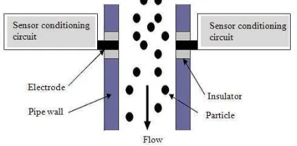
The electrodynamics sensor is a very important part of the electrical charge tomography system. The purpose of the electrodynamics sensor is to capture the electrical charge from the conveyed material such as plastic beads that pass through the sensor/transducer (Furati et al., 2005; Ali and Khamis, 2005; Addasi, 2005). The electrodynamics sensor consists of a plain metal rod called electrode, which is isolated from the walls of the metal conveying pipe by an insulator e.g. glass or plastic. Supported by signal conditioning circuits, the charge detected by electrodynamics sensor will be changed into voltage and sent to the image reconstruction system (computer system) through the data acquisition system. The magnitude of the charges `depends on many factors such as the physical properties of the particles including shapes, sizes, density, conductivity, permittivity, humidity and composition (Yan et al., 1995). The cross-section (Zhao, 2005) of two electrodynamics sensors installed in the pipe is shown in Fig. 1.
The charge conditioning circuit can be designed such that to detect the charges from the moving particles in the conveyor pipeline. Figure 2 shows the block diagram of charge conditioning circuits for an electrodynamics sensor. It consists of several parts i.e., an electrode/electrodynamics sensor, an amplifier (Mou et al., 2004), a rectifier, a low-pass filter and outputs.
Fig. 2: A block diagram of an electrodynamics sensor conditioning circuit
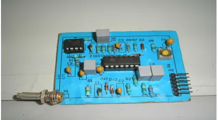
Fig. 3: Electrodynamics sensor fabricated on printed circuit board
Detailed functional discussion of a complete circuit of electrodynamics can be found in (Rahmat et al., 2009a; Ma and Yan, 2000; Machida et al., 1996).
In Fig. 2, output 1 is an alternating component of the charge signal-AC signal used for velocity measurement. Output 2 is the rectified voltage, which can be used for spatial filtering test. Lastly, output 3 is a signal without concern for frequency called DC averaged voltage and is used for concentration measurement and flow regimes identification (Rahmat et al., 2009b). Output 3 is the signal of interest for the proposed system.
Figure 3 shows an electrodynamics sensor with conditional circuit mounted in printed circuit board. The electrode is a silver steel rod on the left of Fig. 3. Other 6 pin connectors on the right of Fig. 3 are connection to the power supply (from the bottom +12 V, ground and -12 V) and outputs (from the top Output 1, 2 and 3) respectively. When installed in the system, the electrodes are isolated from the pipe wall using insulator.
Methods: EChT image reconstruction process involves
two problems which have to be solved i.e., forward modeling problem solution and inverse problem solution.
Fig. 4: Two and three-dimensional total sensitivity map In electrical charge tomography, imaging forward modeling is pre-described as the theoretical of the system in sensing area. It is related to sensor’s sensitivity to the three-dimensional charge, which contains a uniformly distributed charge in coulomb per cube meter (C m−3). Process tomography system by electrical charge is given one measurement from each of the sensors; the amount of information available is equal to the number of the sensors (Rahmat et al., 2010). Therefore, forward modeling of the pipe and the sensing area are mapped equally to the number of the sensor i.e., sixteen by sixteen-rectangular array consisting of 256 pixels or elements. The length between sensors is divided equally and located around the pipe at respective coordinates (Isa and Rahmat, 2008). The sensitivity matrix S derived from the modeling and the summation of complete sensitivity for sixteen sensors in two and three-dimensional is shown in Fig. 4.
Inverse problem is the solution that provides an image of the charge concentration distribution within the sensing area. In order to solve the inverse problem better, a systematic approach of image reconstruction algorithm is very important. Even though the image reconstruction had been discussed by many researchers (Yan and Byrne, 1997; Machida and Scarlett, 2005; Rahmat et al., 2010; Yan et al., 1995), but in EChT system, this aspect is still much to be explored.
1257 value of concentration is reduced away from the sensor location to the center of sensing area (Rahmat et al., 2010). The problem with LS method is no unique solution (Isa and Rahmat, 2009). In addition, these methods normally faced with ill-posed problem. This is because sensitivity matrix or coefficient matrix used in EChT is ill-posed. This situation posts difficulties to the inverse problem solution especially in terms of accuracy and stability of the image being reconstructed (Isa and Rahmat, 2008). In order to ensure stability and accuracy, a special solution should be applied as to obtain a meaningful image reconstruction result. As a result, the least square and regularization techniques are proposed.
A common way to solve Eq. 2 is to generate the estimated value of q as the Least Square (LS) solution to the set of Eq. 3:
Min|| Sq-V||2 (3)
With solving Eq. 3, then:
qLS = (STS)-1 STV (4)
The solution in Eq. 4 is not unique. This is because the matrix (STS)-1 is not invertible. This is because the matrix sensitivity being used is ill posed. Hence, the Singular Value Decomposition (SVD) is a superior numerical ‘tool’ for analysis of discrete ill-posed problem (Hansen, 2007). The SVD will reveal all the difficulties associated with the ill-conditioning of the matrix. Ill-posed problem needs to have conditions numbers as high as 1×10²⁰ (Isa and Rahmat, 2008). In this equation S is the matrix sensitivity produced in forward modeling. With M X N as the rectangular matrix where M≥N, then the SVD of S is a decomposition of the form (5) (Hansen, 1992b):
Min(m,n) T i i i i =1
S =
∑
uσv (5)Where:
Ui = (u1,…….un)
Vi = (v1…….vn) are matrices with orthonormal columns
UTU = VTV = In Where:
∑ = diag(σi…..σn)
σi = The singular values of S
Ui and Vi = The left and right singular vectors of S
(a)
(b)
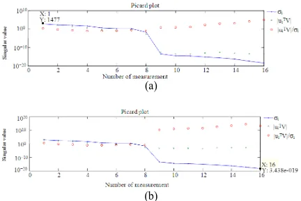
Fig. 5: Discrete Picard chart for LS solution (a) unperturbed from noise error (b) perturbed from noise error
The condition number is equal to the ratio of σ1 and
σn (first and last positive numbers of singular value). From (4), the solution can be formulated by using SVD to check the level of ill-posed of (4) used in EChT. Therefore, Eq. 6 is formulated (Hansen, 2007):
T k
i
ls i
1 i
u V
q = v
σ
∑
(6)
Denoted as V, the data measured in the system. uTi and vi are the left and right singular vectors, while σi is the singular value of S. Discrete Picard Condition (DPC) chart is used to compare between the decay of Fourier coefficients |uiTV| and the singular value σi. If the decay of |uiTV| is faster than the singular value σi, then the solution is acceptable or accepted as a stable solution. Besides that, the solution to the problem is imposed with ill-posed problem (Hansen, 2007).
Figure 5a and 5b respectively shows the DPC produced by the system for unperturbed and perturbed data from noise error. In Fig. 5a, most of the Fourier coefficients |uiTV| for the unperturbed problem satisfy the DPC. However, in Fig. 5b, it can be seen that when the sample data was perturbed by noise error the decay of the singular value is faster than the Fourier coefficients |uiTV|. It can also be noticed that it’s not a stable solution and imposed with ill-posed problem.
imposing additional information about the solution. A penalty term can be added to the optimization problem as (7) below:
E(q) = argmin||Sq-V||2+ß2||R(q-qo)||2 (7) A simple choice for the regularization penalty term is Tikhonov regularization (Soleimani, 2005). The aim of this regularization is to dampen the contribution of the small singular value in the solution. The matrix R is a regularization matrix, which penalizes extreme changes in parameter q and removes the instability in the reconstruction. The parameter ß is called regularization parameter. The solution of (7) would be written in a simple form of the Standard Tikhonov (ST). When R = I and by assuming qo = 0, then (8) is being introduced:
qST = (S T
S+ß2I)-1STV (8)
From (8), the solution can be formulated by using SVD to compare the level of ill-posed of (8) used in EChT. Therefore, Eq. 9 is formulated (Hansen, 2007):
T k
i i
ST 2 2 i
1 i i
u V
q . v
( ß ) σ =
σ + σ
∑
(9)
Figure 6a and 6b show the DPC produced by the system for (9). Figure 6a shows that the Fourier coefficients |ui
T
V| for the unperturbed problem satisfy the discrete Picard condition. In Fig. 6b, it can be seen clearly that even when the sample data was perturbed by noise error, the decay of coefficients Fourier |uiTV| is still faster than the singular value and there was no changes even though the noise was affected at the measurement data.
(a)
(b)
Fig. 6: Discrete Picard chart for ST method (a) unperturbed from noise error (b) perturbed from noise error
The condition number obtained from this solution is 143.52 (first and last singular value is 76.87 and 0.5356). It shows that with regularization the stability of the image becomes much better than the LS solution approach. This is because the regularization solution possesses the filter factor that dampens or filters out the contribution of a small singular value to the solution. The regularization solution is also capable of regulating the solution in a stable manner. The filter factor fi is defined as (10):
i
i 2 2
i f
( ß ) σ =
σ +
(10)
The important property of this filter factor is that it tends to move to zero as σi decreases in such a way that the contribution (uTiV/σi)vi to the solution from the smaller σi is effectively filtered out (Hansen, 2007).
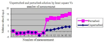
In term of accuracy of the both least square and regularization solution (ST), the sixteen values of solution |uiTV|/σi for qls and qST are plotted as shown by Fig. 7 and 8.
For comparison the solution values of unperturbed and perturbed data with noise for LS method as shown in Fig. 7, which is the solution values for data number 1 until number 8 is almost similar.
Fig. 7: The graph for least square solution value versus number of measurements
1259 (a)
(b)
(c)
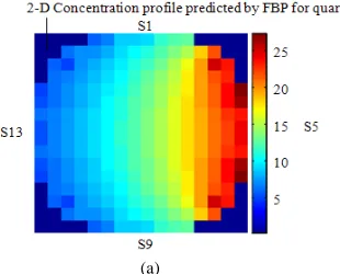
Fig. 9: Image being compared (a) Image reconstructed by FBP (b) Image reconstructed by ST (c) Image reconstructed by LSR
However, the values are exponential increased whenever solution reached at data number 9-16. Its shows that the solution produces by LS method are inaccurate and also cause unexpected or unpredicted solution when reach at certain number of measurements. Otherwise, in Fig. 8 the solutions which is imposed with regularization (ST) it can be seen that the solution values for unperturbed and perturbed data with noise is almost similar for all sixteen measurements of data and the absolute error value is around 0.018%. Thus it shows that with regularization
(ST), the solutions is more accurate and remain accurate although the numbers of measurements is increased.
However, for the described algorithm in (8), the choice of regularization is important. In general, a small value of ß gives a good approximation to the original problem but the influence of errors may make the solution physically unacceptable. Conversely, a large value of ß suppresses the data but increases the approximation error. At present and in most cases, ß are chosen empirically. The value of regularization parameter of 0.025908 is obtained (Rahmat et al., 2009b).
The advantage of Eq. 8 is that it can detect two or more charges at separate points in sensing area but it has ghosting image at adjacent points. However, filtered back projection (qFBP) is accurate in detecting the area of the charge but it cannot distinguish between the two separate charges in the sensing area (Isa and Rahmat, 2009). Therefore, the best way to solve the problem of image reconstruction process is by using qFBP and Standard Tikhonov (ST). As a result, (11) is used to produce the image concentration in the sensing area (Jadan and Addasi, 2005). This method is called the least square with regularization method (qLSR):
qLSR = qFBP FilterST (11)
where, the FilterST obtained by taking each value (qSTi) of pixel in qST, divided by the maximum value of pixel (qSTmax) in qST. Figure 9 shows the different images being compared that have been reconstructed by qFBP, qST dan qLSR methods in Fig. 9a-c respectively. The advantage of qLSR as shows in Fig. 9c is that it can detect two charges at separate points in the sensing area and as accurate as FBP method.
RESULTS
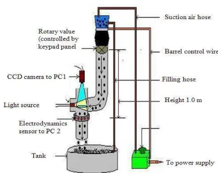
Fig. 10: Experiment apparatus for data capturing process
It is quite a simple matter to focus a CCD camera on this system and acquire the digital images. Figure 10 illustrates the experimental apparatus used in the validation process.
The materials used in this system are the 3 mm-size plastic bead particles. The data measured by the electrodynamics sensor are recorded within the same as ten seconds period as recorded by CCD camera. The CCD camera will capture video of materials moving through the pipe hole, sent and store it to the computer system 1 (PC 1). The sizes of the pictures are 1000×1000 pixels. Meanwhile, the electrodynamics sensor will be induced by the charge from the material that passes through the sensors. This charge will be converted into voltage by the electrical conditioning circuit attached to the sensor. The voltage will be sent and store to the image reconstruction system (computer system 2-PC 2) via Keithely STA-1800HC data acquisition card. Image reconstruction process has been done off line using MATLAB programming language based on LBP, FBP and LSR methods. On the other hands, video recorded by CCD camera in computer PC 1 will process using digital image processing to produces single image concentration profile for material being drops in pipeline. Finally, images reconstructed will be compared to the images captured by the CCD camera. Verifying process of the images reconstructed is based on their similarity to the images produced by CCD camera. Figure 11 shows the three different modes of image captured by the CCD Camera.
Figure 12 shows the images reconstructed by LBP, FBP and LSR being compared to image captured by CCD camera. These images based on data measured by electrodynamics sensor at the same time when CCD camera recorded the video (as shown in Fig. 11).
(a) (b) (c)
Fig. 11: Images recorded by CCD Camera (a) image with absolute value and threshold (b) image with identified sensing area (c) real image resized to 16×16 pixels with color mode
(a) (b) (c)
Fig. 12: Images being compared (a) Image reconstructed by LBP (b) image reconstructed by FBP (c) image reconstructed by LSR method
DISCUSSION
Figure 11a shows the original image of material flown in the pipeline as captured by CCD camera. Figure 11b is the image with identified sensing area in grey and Fig. 11c is the image of Fig. 11b after being resized to 16×16 matrixes and converted to color mode using MATLAB.
Figure 11c shows the image captured by the CCD camera with the highest image concentration area as shown in circle and labeled as A. The other high concentration areas shown in circles are labeled as B and C. In addition, for every high concentration area there are many different values of concentration in each pixel. This means that in real situation the particles dropped in conveyor pipeline are scattered around the pipe with many concentration zone areas but at different value of concentration and with a lot of charges present in the sensing zone area.
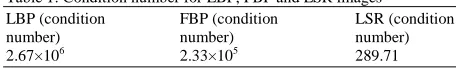
1261 Table 1: Condition number for LBP, FBP and LSR images
LBP (condition FBP (condition LSR (condition
number) number) number)
2.67×10⁶ 2.33×10⁵ 289.71
In Fig. 12a, image pattern reconstructed using LBP method shows that the image concentration are not focusing on the area as shown by the real image recorded using CCD camera as in Fig. 11c. Instead, the high concentration values focus on the sensor (the edge of sensing area) itself. This means that LBP method is not suitable in reconstructing the image for electrical charge tomography due to of its non-linearity to the sensing mechanism.
Figure 12b shows the image reconstructed by FBP method. The high concentration area focuses around the sensor as recorded in Fig. 11c are labeled A, B and C. The concentration pattern in these zones reduces the value away from the centre. This means that FBP detects more charges near the sensor location and reduced away to the centre. In general, the image reconstructed by FBP is accurate in detecting the high concentration zone area but the pattern is not similar to the image recorded by CCD camera. As a result, FBP method cannot produce images similar with the images produced by CCD camera. Thus, FBP is not applicable to be used in industrial process.
Figure 12c shows that the pattern for high concentration area for LSR method is scattered with different value of concentration. There are many pixels with different values of concentration in the sensing zone areas as labeled A, B and C. This means that the image reconstructed by LSR method has the capability to differentiate between zone areas and pixels with high value of concentration within the same zone area. For comparison, it shows that the zone area and pattern of concentration reconstructed by LSR method is similar to the image recorded by the CCD camera as shown in Fig. 12c.
Analysis of condition number of the images has been performed using the Singular Value Decomposition (SVD) method. Table 1 shows the condition number of ill-posed for each method.
From the results, it shows that LSR method produces the lowest condition number compare to LBP and FBP methods. The result reflects that LSR method produces better image stability than any other methods.
CONCLUSION
The results imply that LSR method provides good and promising result in terms of accuracy and stability of the image being reconstructed. This means that this
study succeeds in achieving its objective mentioned earlier. Therefore, to enable EChT technology be used in real industry environment, more work on hardware and software systems should be carried out to guarantee that their data and algorithm are well organized and developed.
ACKNOWLEDGEMENT
The second author acknowledges the scholarship from the Ministry of Higher Education of Malaysia in Tomography: Principles, Techniques and Application. 1st Edn., Butterworth-Heunemann, USA., ISBN: 10: 0750607440, pp:384.
Bailey, A.G., 1998. The science and technology of electrostatic powder spraying, transport and coating. J. Electrostat., 45: 85-120. DOI:
inverse problem with discrete data: II stability and regularization inverse problem. Inverse Problem, 4: 573-594.
http://cat.inist.fr/?aModele=afficheN&cpsidt=7303 222
Carter, T.M., Y. Yan and S.D. Cameron, 2005. On-line measurement of particle size distribution and mass flow rate of particles in pneumatic suspension using combined imaging and electrostatics sensor. Flow Measure. Instrument., 16: 309-314. DOI: 10.1016/j.flowmeasinst.2005.03.005
Carter, R.M. and Y. Yan, 2003. On-line particle sizing of pulverized and granular fuels using digital imaging techniques. Measure. Sci. Technol., 14: 1099-1109.
Ding, Y.W. and F. Dong, 2007. An image reconstruction algorithm based on regularization optimization for process tomography. Proceeding of the 6th Conference on Machine Learning and Cybernetics, Aug. 19-22, IEEE Xplore Press, Hong
Kong, pp: 1717-1722. DOI:
10.1109/ICMLC.2007.4370424
Furati, K.M., H. Tawfiq and A.H. Siddiqi, 2005. Simulation and visualization of safing sensor. Am. J. Applied Sci., 2: 1261-1265. DOI: Technol., 8: 192-197. DOI: 10.1088/0957-0233/8/2/014 solution of Fredholm integral equations of the first kind. Inverse Problems, 8: 849-872. DOI: 10.1088/0266-5611/8/6/005
Hansen, P.C. and D.P. O’Leary, 1993. The use of the L-curve in the regularization of discrete Ill-posed problems. SIAM J. Sci. Comput., 14: 1487-1503.
Isa, M.D. and M.F. Rahmat, 2008. Image reconstruction algorithm based on least square with regularization for process tomography system using electrical charge carried by particles. Proceedings of the Student Conference on Research and Development, Nov. 26-27, IEEE Computer Society, Malaysia, pp: 1-4.
Isa, M.D. and M.F. Rahmat, 2009. Application of digital imaging technique in electrical charge tomography for image reconstruction validation. Proceedings of the 2nd International Conference on Machine Vision, Dec. 28-30, IEEE Xplore Press, Dubai, pp: 277-281. DOI: 10.1109/ICMV.2009.35 Jadan, M. and J.S. Addasi, 2005. Control of oxygen
concentration by using a carbonaceous substance. Am. J. Applied Sci., 2: 768-770. DOI: 10.3844/ajassp.2005.768.770
Krawczyk-StanDo, D. and M. Rudnicki, 2007. Regularization parameters selection in discrete ill-posed problem-the use of the L-curve. Int. J. Applied Math. Comput. Sci., 17: 157-164. DOI: 10.2478/V10006-007-0014-3
Ma, J. and Y. Yan, 2000. Design and evaluation of electrostatic sensors for the measurement of velocity of pneumatic conveyed solids. Flow Measure. Instrument., 11: 195-204. DOI: 10.1016/S0955-5986(00)00019-4
Machida, M. and B. Scarlett, 2005. Process tomography system by electrostatic charge carried by particle. IEEE Sens. J., 5: 252-259. DOI: 10.1109/JSEN.2005.843892
Machida, M., J.C.M. Marijnissen and B. Scarlett, 1996. Mathematical model for charged particle measurement. J. Aerosol Sci., 27: S205-S206.DOI: 10.1016/0021-8502(96)00175-9
Masuda, H., S. Matsuaka and H. Shimomura, 1998. Measurement of mass flow rate of polymer powder based on static electrification of particles. Adv. Powder Technol., 9: 169-179. DOI: 10.1163/156855298X00137
Matsusaka, S. and H. Masuda, 2003. Electrostatics of particles. Adv. Powder Technol., 14: 143-166. DOI: 10.1163/156855203763593958
Mohamad, D., B.M. Deros, D.A. Wahab, D.D.I. Daruis and A.R. Ismail, 2010. Integration of comfort into a driver’s car seat design using image analysis. Am. J. Applied Sci., 7: 937-942. DOI: 10.3844/ajassp.2010.937.942
Mou, S., Ma J., K.S. Yeo and M.A. Do, 2004. A fully integrated dual-band low noise amplifier for IEEE 802.11 and Hiperlan applications. Am. J. Applied Sci., 1: 26-32. DOI:10.3844/ajassp.2004.26.32 Nifuku, M., T. Ishikawa and T. Sasaki, 1989. Static
Electrification phenomena in pneumatic transportation of coal. J. Electrostat., 23: 45-54. DOI: 10.1016/0304-3886(89)90031-4
Rahim, R.A., C.K. Thiam, M.H.F. Rahiman, J. Pusspanathan and Y.S.L. Susiapan, 2008. Optical tomography system: Digital sensors for masking purpose in parallel beam optical tomography system. Sensor Lett., 6: 752-758. DOI: 10.1166/sl.2008.m157
Rahmat, M.F., M.D. Isa, R.A. Rahim and T.A.R. Hussein, 2009a. Electrodynamics sensor for the image reconstruction process in an electrical charge tomography system, Sensors, 9: 10290-10308. DOI: 10.3390/s91210291
Rahmat, M.F., N.S. Kamaruddin and M.D. Isa, 2009b. Flow regime identification in pneumatic conveyor using electrodynamics transducer and fuzzy logic method. Int. J. Smart Sens. Intell. Syst., 2: 396-416. http://www.s2is.org/Issues/v2/n3/papers/paper3.pdf Rahmat, M.F., H.A. Sabit and R. Abdul Rahim, 2010. Application of neutral network and electrodynamics sensor as flow pattern identified.
Sens. Rev., 30: 137-141. DOI
1263 Soleimani, M., 2005. Numerical modeling and analysis
of the forward and inverse problems in electrical capacitance tomography. Int. J. Inform. Syst. Sci., 1: 193-207. http://www.math.ualberta.ca/ijiss/SS-Volume-1-2005/No-2-05/SS-05-02-08.pdf
Sugita, T., M. Kamimura and Y. Kitayama, 2003. A particles size distribution measuring method for pulverized particle spherically equivalent diameter of the particle floating in the airflow. Proceedings of the SICE Annual Conference, Aug. 4-6, IEEE Xplore Press, USA., pp: 1719-1722. DOI: 10.1109/SICE.2003.1324235
Schein, L.B., 1999. Recent advances in our understanding of toner charging. J. Electrostat., 46: 29-36. DOI: 10.1016/S0304-3886(98)00056-4 Tarantola, A., 2005. Inverse Problem Theory and
Methods for Model Parameter Estimation. 1st Edn., Society for Industrial and Applied Mathematics, Philadelphia, PA., USA., ISBN: 10: 0898715725, pp: 352.
Woodhead, S.R., Denham, J.C. and D. Armour-Chelu, 2005. Electrostatic sensors applied to measurement of electric charge transfer in gas-solids pipelines. J. Phys.: Conf. Ser., 15: 108-112. DOI: 10.1088/1742-6596/15/1/018
Xu, C., S. Wang, G. Tang, D. Yang and B. Zhou, 2007. Sensing characteristics of electrostatic inductive sensor for flow parameters measurement of pneumatically conveyed particles. J. Electrostat., 65: 582-592.DOI: 10.1016/j.elstat.2007.01.001
Yan, Y. and B. Byrne, 1997. Measurements of solids deposition in pneumatic conveying. Powder Technol., 91: 131-139. DOI: 10.1016/S0032-5910(96)03249-4
Yan, Y., B. Byrnet, S. Woodhead and J. Coulthard, 1995. Velocity measurement of pneumatically conveyed solids using electrodynamic sensors. Measure. Sci. Technol., 6: 515-537. DOI: 10.1088/0957-0233/6/5/013
Yang, W.Q. and L. Peng, 2003. Review article: Image reconstruction algorithms for electrical capacitance tomography. Measure. Sci. Technol., 14: R1-R13. DOI: 10.1088/0957-0233/14/1/201
Zhang, Y., Y.C. Liang and C.H. Wang, 2008. Hazard of electrostatic generation in a pneumatic conveying system: electrostatic effects on the accuracy of electrical capacitance tomography measurements and generation of spark. Measure. Sci. Technol., 19: 1-10. DOI: 10.1088/0957-0233/19/1/015502 Zhao, B., 2005. Modeling of particle separation in
bends of rectangular cross-section. Am. J. Applied
Sci., 2: 394-396. DOI: