Dynamic Analysis of Regional Convergence in
Indonesia
MUHAMMAD FIRDAUSa AND ZULKORNAIN YUSOPb*
a Department of Economics, Faculty of Economics and Management,
Bogor Agricultural University, 16680, Bogor, West Java, Indonesia b Department of Economics, Faculty of Economics and Management,
Universiti Putra Malaysia, 43400, Serdang, Selangor , Malaysia
ABSTRACT
This study examines income convergence among provinces in Indonesia using dynamic panel data approach. The results show that static and dynamic panel data approaches produce different results of convergence patterns. Consistent with the theory, the Ordinary Least Square (OLS) and fixed-effects estimators provide the upper and lower bounds. The first-differences generalized method of moments (FD-GMM) provides invalid estimators which are lower than the coefficient from the fixed effects estimators due to the weak instruments problem. The system-GMM (SYS-GMM) estimators are found to be unbiased, consistent and valid. They show that convergence process prevails among provinces in Indonesia for the period 1983 – 2003. However the speed of convergence is relatively very slow (0.29) compared to other studies in developing countries.
Keywords: Dynamic Panel Data, Income Convergence and Indonesia.
INTRODUCTION
Some tactical policies related to regional development, were implemented in Indonesia since the early 1970s. They were aimed to promote a more balanced regional development. From the iscal perspective, expanded iscal revenue during the oil boom in 1970s enabled the transfer of massive resources to islands that were heavily relied on suffering non-oil export sectors. Massive resources were transferred through a government-based channel, which contributed to
* Corresponding author: E-mail: zolyusop@econ.upm.edu.my
developing regional infrastructure, such as roads, schools and health facilities. They were represented in government expenditure from budget allocation of central government into provinces. Some remarkable social progresses were made in this period. Moreover, some tactical programs were intended also to achieve more equitable regional development, such as INPRES (Instruction of President) program for least developed villages. It was part of iscal decentralization policy that allowed regional governments to have greater autonomy in reducing poverty (Takeda and Nakata, 1998).
However, an increasing level of regional income inequality (despite the rapid economic growth) suggests that some of the above policies are ineffective. This regional disparity is also indicated by the coeficient of variation (CV) for per capita GDP among provinces compared to some developing countries. In 1997, it was 0.83 while the other developing countries varied from 0.186 to 0.797. Shankar and Shah (2001) also reported that developing countries were much more unequal than the developed ones. A study using Theil index based on GDP and population data (Akita and Alisjahbana, 2002) reported that overall regional income inequality increased signiicantly over the 1993 – 97 period (from .262 to .287), during which time Indonesia achieved an annual average growth rate of more than 7 percent. The increase was due mainly to a rise in the within-province inequality component, especially in the provinces of Riau, Jakarta, West Java and East Java. The between-province inequality increased but only very slightly.
The regional disparity in Indonesia represents an ever-present development challenge in most countries with large geographic areas. Globalization heightens these challenges as it places a premium on skills. With globalization, skilled labors rather than the availability of resources in the regions are more important in terms of competitiveness. As rich regions have more educated and skilled labor, the gap between rich and poor regions widens. Poor regions become poorer and the rich ones become richer. However, neoclassical models posit that regions with low capital-labor ratios should catch up to the level of the developed regions because of the higher marginal productivity of a unit capital invested. For many policy considerations, this regional convergence and reduction of regional disparity is indeed very important and deserved attention. Thus, it is the objective of this study to investigate whether the Indonesia’s regions converge? If so, what is the speed of the convergence? The rest of this article consists of ive sections i.e. review of previous empirical studies; method and data; analysis and estimation; results and discussion; and inally conclusion and policy implication.
PREVIOUS EMPIRICAL STUDIES
the estimation of conditional convergence was soon criticized for econometric reasons: the initial level of technology, which should be included in a conditional convergence speciication, is not observed. Since it is also correlated with another regressor (initial income), all cross section studies suffer from an omitted variable bias. Islam (1995) proposed to set up convergence analyses in a panel data framework where it is possible to control for individual–speciic, time invariant characteristics of countries (like the initial level of technology) using ixed effects. However, the coeficient from this estimation tends to show a downward bias in the dynamic panel (Badinger, 2002). An upper bound for the coeficient of the lagged endogenous variable is provided by the simple pooled OLS-estimator of a panel data model, which is seriously biased upwards in the presence of ixed effects.
The problems and weaknesses associated with cross-sectional test have led certain researchers to consider time-series approaches as alternative (Bernard and Durlauf, 1995). Time-series approach requires that the long run equilibria for the economies under studied not very far from each other since the tests assume that the sample moments of the data accurately approximate the limiting moments for the data under analysis. In other word, the former appears to more naturally apply to the transition data. Whereas the later appear to more naturally apply to the data which sample moments well approximate the properties of the limiting distribution of the economies under the study. Consequently, a given approach is appropriate depending upon whether one regards the data as better characterized by transition or steady state dynamics.
Given this recent developments in convergence analysis, the ideal approach would be to combine both viewpoints in a spatial dynamic panel data model in order to meet the underlying arguments of both approaches. The panel data method is currently perceived as the best available, irst-differenced and system generalized method of moments (GMM), which could produce the reasonable parameter estimates that lie within the range of OLS and ixed estimates.
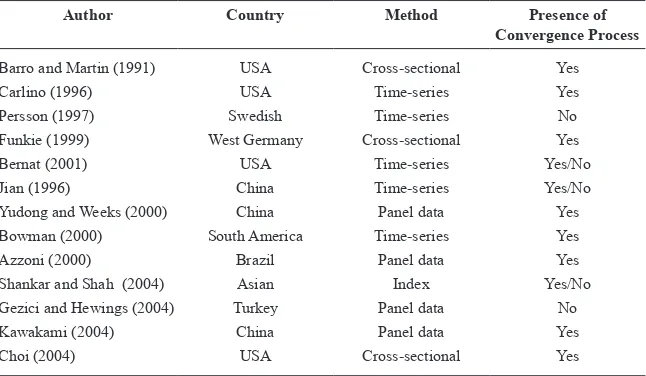
Table 1 summarizes some studies of income convergence among regions within a country.
Table 1 Some indings of convergence process within a country
Author Country Method Presence of
Convergence Process
Barro and Martin (1991) USA Cross-sectional Yes
Carlino (1996) USA Time-series Yes
Persson (1997) Swedish Time-series No
Funkie (1999) West Germany Cross-sectional Yes
Bernat (2001) USA Time-series Yes/No
Jian (1996) China Time-series Yes/No
Yudong and Weeks (2000) China Panel data Yes
Bowman (2000) South America Time-series Yes
Azzoni (2000) Brazil Panel data Yes
Shankar and Shah (2004) Asian Index Yes/No
Gezici and Hewings (2004) Turkey Panel data No
Kawakami (2004) China Panel data Yes
Choi (2004) USA Cross-sectional Yes
EMPIRICAL METHOD
There are two critical issues in testing the convergence hypothesis. First, is there evidence of convergence process? The second issue is related to the consistency of the convergence estimate. This study uses the Solow growth model to resolve both issues. Following Mankiw et al (1990), we assume constant returns to scale Cobb-Douglas production function with output (Y) and three inputs, capital (K), labor (L) and labor augmenting technological progress (A)
Y t K t A t L t 1
= a -a
^ h ^ h^ ^ h ^ hh (1)
where 0 < α < 1. Labor force and technology grow at the following constant and exogenous rates
L t^ h=L^0hent
(2)
A t^ h=A^0hegt
(3)
If y t
where s is the savings rate and d is the depreciation rate of capital. Capital is subject
to diminishing marginal returns such that
( )
steady state capital stock, kt*
, can be determined by setting equation (4) equal to zero output per effective unit of labor can be derived, which in logarithmic form may be written
Around the steady state, the rate of convergence, λ, denoting the rate at which output per effective unit of labor approaches its steady state value, is given by
ln ( )
The solution of the differential equation (7) is
ln ( )y t (1 ) lny* (1 ) ln ( )y t
2 = -w + -w 1
t
t
t
(8)where w=emx
, and x=(t2-t1). This equation represents a partial adjustment
process where the optimal target value of the dependent variable is determined by the explanatory variables of the current period. In the present case, y
t
*If now output is measured in per effective unit of labor, equation (8) can be
= stands for capita output, and the parenthetical term z denotes
the log of the steady- state per capita output.
Let b= -(1-w) denote the parameter on income at t1, the speed of convergence
is the given by
ln ( 1)
m= - bx+ (11)
Equation (10) can be written as an autoregressive form of the growth model
ln ( ) ln ( ) ( ) ln ( ) ( )
Here the effects hi can be interpreted as a composite of unobservable
province-speciic factors, thereby representing the combined effect of institutions, factor endowments, and relative location, together with the initial technology differences.
νit error-term which is assumed IID (0,σ2). In this study, the inal equation of testing convergence hypothesis that is estimated as follow
( ) '
zit 1 a zit 1 b xit Di uit
D = - D - + D + +D (14)
i = 1, 2, ..., N and t = 3, ..., T
where z is regional income and xit consists of investment-ratio to regional GDP; population growth rate + technological progress rate + depreciation which is assumed 5 percent. This is similar to some previous studies and growth literature
(Romer, 2006). The convergence process prevails if the coeficient of (1- α) is
less than one. The rate of convergence is counted as – ln (α).
DATA AND ESTIMATION PROCEDURE
This study uses the data of provincial gross domestic product for without and with oil and gas sector; value of domestic and foreign investment; number of population and assumption of g+κ= 0.05 from 1983 up to 2003. In estimation, the three-year average data is used. There are 26 provinces involved in this study. All data are real and measured in 1993 prices.
In estimating the dynamic panel data model, equation (14) is known as dynamic panel regression i.e. a panel regression with lagged dependent variable on the right-hand side. Following Arellano and Bond (1991); Arellano and Bover (1995), the above issue can be addressed under a Generalized Method of Moments (GMM) framework.
Application of GMM irst differences estimator requires
lnYit c lnYi t, 1 bln xit ni ht yit
D = D - + D +D +D +D (15)
for t = 3, ..., 7 and i = 1, ..., 26
where yit-2 and all previous lags are used as instruments for ∆yit – 2 assuming that
E[νitνis] = 0 for i = 1, ..., N and t ≠ s and exploiting the moment conditions that denoted by E[yit – sνis] = 0 for t = 3, ..., 7 and s ≥ 2. However, the GMM estimator
lnYit=clnYi t,-1+b1lnxit+ni+ht+yit (6)
for t = 2, …, 7and i = 1, ..., 26
Estimation of the model employs a modiied program of dynamic panel data (DPD) created by Kitazawa (2003).1
RESULTS AND DISSCUSSION
Results of panel data estimation procedures are reported in this section. Table 2 shows the comparison of OLS, ixed effects, random effects estimators and dynamic panel estimators (FD-GMM and Sys-GMM). The OLS provides a high estimate of the coeficient of autoregressive parameter, γ. The coeficient of yi,t-1 is greater
than one means that the provincial income is highly persistent. It implies the convergence process does not prevail among provinces in Indonesia. This result may be due to a bias arising from the model speciication that does not adequately allow for unobserved differences across countries or regions. Table 2 also shows that the sign of the coeficient of investment-GDP ratio (sit) is positive and statistically signiicant at 5 percent level. It is consistent with the theory. This indicates that foreign investment plays an important role in regional development of Indonesia. The coeficient of population growth + depreciation (xit) is positive which is not consistent with theory. However the p-value of such coeficient is greater than .05 that means the coeficient is not statistically signiicant.
The choice between ixed and random effects as a correct model in static panel data estimation needs Hausman test. Hausman test statistic (X2) is 48.307 which
means that the null hypothesis of random effects as a correct model is rejected or the ixed effects model is a correct model. Indeed the parameter estimated by using ixed effects model can be used as lower bound parameter for the dynamic panel data selection and the ixed effects estimators are the most robust among the static panel data estimates.
The ixed effects estimator provides a lower estimate of the coeficient of autoregressive parameter than OLS. The coeficient of yi,t-1 is .8817 or less than
one. This indicates that the (conditional) convergence process persists among provinces in Indonesia. The implied speed of convergence based on this result is about 12.6 percent. This speed is likely the same as the results reported by other convergence studies that employ ixed effects procedure. For example, Fuente (1996) inds a convergence rate of about 10 percent fro Spanish regions. All signs of the coeficients of regressors are consistent with the theory. The coeficient of investment-GDP ratio is positive but not statistically signiicant at 5 percent level.
1 The sample of program can be obtained from http://www.ip.kyusan-.ac.jp/J/keizai/kitazawa/SOFT/
The coeficient of population growth + depreciation is negative and statistically signiicant at 5 percent level. The ixed effects model is also it as indicated by a high adjusted coeficient of determination.
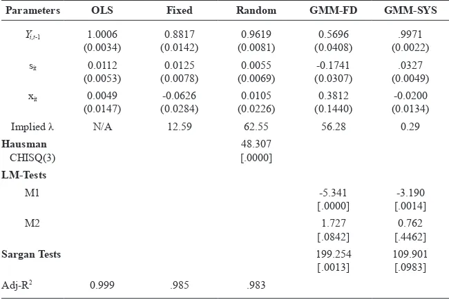
Table 2 Results of estimation for income convergence in Indonesia
Parameters OLS Fixed Random GMM-FD GMM-SYS
Yi,t-1 1.0006
Implied λ N/A 12.59 62.55 56.28 0.29 Hausman
Notes: LM test is a test for irst-order and second-order serial correlation in the irst-differenced residuals, asymptotically distributed as N(0,1), under the null of no serial correlation. Sargan test is a test of the over-identifying restrictions, asymptotically distributed as χ2 under the null of instrument validity. The igures in the bracket [ ] denote a
p-value.
The alternative model of the static panel procedure is random effects model. The lagged coeficient is higher than the ixed effects estimate, but still less than one. This convergence process prevails with the high speed of 62.5 percent. Indeed this proves that the ixed effects estimate suffers from a serious downward bias. The sign of investment-GDP ratio is positive but not statistically signiicant at 5 percent level. However the sign of population growth + depreciation is positive, which is not consistent with the theory. The random effects estimation model is also it. The model has a high adjusted R2 of 98.32 meaning that 98.32 percent of
variation in explanatory variables can be explained by the variation in dependent variable.
(Judson et al., 1999). Although this bias tends to be zero as T approaches ininity, it cannot be ignored in small samples. Using Monte Carlo studies, Judson et al. ind that the bias can be as large as 20 percent even for fairly long panels with
T = 30. However both OLS and random effects estimate provide the lower and upper bound parameter estimated from the dynamic panel data model. Thus the dynamic panel data estimation of irst differenced GMM (FD-GMM) and system GMM (SYS-GMM) are employed in this study to ind the prevailing and the precise speed of convergence process.
Table 2 presents the parameter estimates using the FD-GMM estimator, with assumption of initial income, investment and population growth being endogenous. The coeficient on the lagged dependent variable is positive and statistically signiicant at 5 percent level. The coeficient of yi,t-1 is less than one implying the convergence process prevails among provinces in Indonesia. It is much lower than the random effect estimate. Thus it gives a higher speed of convergence of 56.28 percent. Both The coeficient of investment-GDP ratio and population growth + depreciation is statistically signiicant at 5 percent level. But the sign of investment coeficient is not consistent with the theory. While the coeficient of population growth + depreciation is consistent with the theory.
However the coefficient of the FD-GMM estimator may even be more downward biased than the ixed effects in the case of weak instruments. The GMM estimator in irst differences has been criticized in the literature. As shown by Bond et al. (2001) an indication for weak instruments might be that the coeficient
obtained with the FD-GMM being close to or lower than the coeficient from the ixed effects estimator as reported.
Furthermore an application of Sargan test suggests that the instrumental variables used in the FD-GMM are not valid. The Sargan test shows the rejection of null hypothesis of valid instruments indicated by upper tail area of .0013. An upper bound for the coeficient of the lagged independent variable is provided by the simple pooled OLS-estimator of a panel data model, which is seriously biased upwards in the presence of ixed effects. A plausible parameter estimate should lie between the ixed effects and the OLS estimators. The result can be obtained by using the SYS-GMM.
Table 2 also reports the estimation results from employing the SYS-GMM. Here the estimate of the coeficient on the lagged dependent variable lies comfortably above the corresponding ixed effects estimate, and below the corresponding OLS estimate. The signiicant m1 statistic (.0014) and insigniicant m2 (.4462) statistic
indicate the lack of second order serial correlation in the residuals of the differenced speciication.
that there is indeed a serious inite sample bias problem caused by weak instruments in the FD-GMM results, which can be addressed by system GMM.
Importantly, the unbiased, consistent and valid SYS-GMM estimators also suggest that the investment has a signiicant positive effect on the steady state level of per capita GDP, which is consistent with the theory. This means that the (foreign) investment inlows play a signiicant role in the convergence process. The negative sign of population growth + depreciation is also consistent with the theory, but is not statistically signiicant at 5 per cent level.
The lagged parameter of the SYS-GMM estimate is .9971. The less than one coeficient means that the convergence process prevails among provinces in Indonesia. It implies a speed of convergence of .29 per cent a year. This means that it takes more than 200 years for a typical region to reduce its income gap with the national average by one half. This speed is extremely slow compared to the panel model indings. An examination of income convergence among China’s provinces (Yudong and Weeks, 2000) is the most similar with this study. In that study, China is divided into interior and coastal zones. The best panel data model found that the convergence rate is 2.23 percent for the reform period (1978 – 1977). A cross-sectional study of income convergence among provinces in Indonesia has found that the convergence rate is about 3.13 percent during 1975 – 1993 (Garcia and Soelistianingsih, 1998).
Some reasons for this relatively low rate compared to previous studies are: (1) the existence of decreasing returns to scale in capital in production technology is not fully satisied. This is shown by a positive relationship between growth in regional income and growth in capital; (2) provinces differ in the intensity of their efforts to generate or adopt new technologies. This is indicated by the highly skewed of foreign investment inlows and (3) provinces differ in level of structural change indicated by the faster structural change process in Java island.
To reduce the regional imbalances, some policies have been formulated in 1990s to reduce regional disparities in Indonesia (Takeda & Nakata, 1998). However, they are more in normative level than implementation such as to:
develop infrastructure in less developed regions and stimulate private sector •
investment to build the regional characteristic industries;
provide iscal transfer to local governments in due consideration of disparities •
and characteristics, and
enhance the administrative capabilities of regional government by strengthening •
the human resource development.
The people outside of Java believe that power is not distributed fairly. This state of affairs among regions and rising in poverty rate has stimulated public discussion of the equity issue and driven public policy in Indonesia which resulted in Law No. 22/1999 on regional autonomy and Law No. 25/1999 on iscal equalization between center and regions. They came to effect on January 1, 2000, which were aimed to achieve more equitable growth. However the early regional income data still show signiicant imbalance. For example, per capita GDP of some provinces such as North Sumatra, Jakarta and East Borneo remain above the average Indonesia per capita GDP, on the other hand the poor region such East Nusa Tenggara and Maluku earned only about one fourteenth of the richest province (Jakarta), which remained below a half of average Indonesia per capita GDP.
As a serious disparity problem still arises among provinces in Indonesia, some stronger policies are needed, for example:
Central government should continue and strengthen their local autonomy •
program as serious disparity problem arises among provinces in Indonesia.
Investment is proven to play important role to overcome the regional disparity •
problem. Some remote areas and KTI should be given the greater incentives because the regional policy has not been yet effective to attract the foreign investors. They are tax-preference policy; land-use preferential policy; increasing government investment and expanding areas of foreign investment in remote areas and KTI.
Infrastructure buildings and education program improvements in remote areas •
and KTI must obtain more attention from central government.
CONCLUSIONS
This study conducts some appropriate methods to test the convergence hypothesis. Based on the SYS-GMM, the regional income convergence prevails, but the speed of convergence process is very slow (0.29 percent). This very low speed of convergence process in Indonesia may be related to some reasons, such as increasing rate of returns in capital, imbalances in technological process and structural change of economic development. While these indings may be robust, there are several extensions that should be pursued:
Further research on existing panel data methods of testing convergence •
hypothesis that employs a longer period and the most up to date data should be carried out.
REFERENCES
Akita, T. and Alisjahbana, A. (2002) Regional Income Inequality in Indonesia and the Initial Impact of the Economic Crisis, Bulletin of Indonesian Economic Studies, 38, 201 – 22. Akita, T. and Lukman, R.A. (1995) Interregional Inequalities in Indonesia: A Sectoral
Decomposition Analysis for 1975 – 92, Bulletin of Indonesian Economic Studies, 31, 61 – 81.
Arellano, M. and Bond, S. (1991) Some Tests of Speciication for Panel Data: Monte Carlo
Evidence and an Application of Employment Equations, Review of Economic Studies,
58, 277 – 297.
Arellano, M. and Bover, O. (1995) Another Look at the Instrumental Variable Estimation
of Error-Components Models, Journal of Econometrics, 68, 29 – 51.
Badinger, H., W.G. Muller and Tondl, G. (2002) Regional Convergence in the European Union (1985 – 1999): A Spatial Dynamic Analysis, HWWA Discussion Paper No. 210. Baltagi, B.H. (2008) Econometric Analysis of Panel Data, Third Edition. Wiley: New
York
Barro, R.J. and Martin, X.S. (1991) Convergence Across States and Regions, Brooking Papers on Economic Activity, 1, 107 – 182.
Berg, H.V. (2001) Economic Growth and Development, McGraw-Hill International
Edition.
Bernard, A.B. and Durlauf, S.N. (1994) Interpreting Tests of the Convergence Hypothesis, NBER Working Paper Series No. 159.
, (1995) Convergence in International Output, Journal of Applied Econometrics, 10, 97 – 108.
Bond, S., Hoefler, A. and Temple, J. (2001) GMM Estimation of Empirical Growth Models,
Paper at Department of Economics, University of Bristol, UK.
Bond, S. and Blundell, R. (1998) Initial Condition and Moment Restrictions in Dynamic Panel Data Models, Journal of Econometrics, 87, 115 – 143.
Fuente, A. (2002) On the Sources of Convergence: A Close Look at the Spanish Region,
European Economic Review, 46, 569 – 599.
Garcia, J.G. and Soelistianingsih, L. (1998) Why Do the Differences in Provincial Income Persists in Indonesia? Bulletin of Indonesian Economic Studies, 34, 95 – 120.
Hadi, S. (2001) Studi Dampak Kebijaksanaan Pembangunan terhadap Disparitas Ekonomi antar Wilayah, Ph.D Thesis, Bogor Agricultural University, Indonesia.
Hayashi, F. (2000) Econometrics. Princeton University Press: USA. Hsiao, C. (2004) Analysis of Panel Data. Cambridge University Press: UK.
Islam, N. (1995) Growth Empirics: A Panel Data Approach, The Quarterly Journal of Economics, 110, 1127 – 70.
Shankar, R. and Shah, A. (2001) Bridging the Economic Divide within Nations: a Scorecard on the Performance of Regional Development Policies in Reducing Regional Income Disparities, World Bank Working Papers Series.
Takeda, T. and Nakata, R. (1998) Regional Disparities in Indonesia, OECF Research Papers 23.
Verbeek, M. (2004) Modern Econometrics. John Wiley and Sons Inc.: USA.