accredited by DGHE (DIKTI), Decree No: 51/Dikti/Kep/2010 37
An Efficient Simulated Annealing Algorithm for
Economic Load Dispatch Problems
Hardiansyah1, Junaidi, Yohannes MS
Department of Electrical Engineering, University of Tanjungpura, Pontianak 78124, Indonesia
1e-mail: [email protected]
Abstrak
Makalah ini menyajikan suatu algoritma simulated annealing (SA) yang efisien untuk penyelesaian masalah economic load dispatch (ELD) pada sistem tenaga listrik. Filosofi melibatkan pengenalan variabel keputusan baru melalui transformasi matematika secara bijaksana hubungan antara variabel keputusan dan pembangkitan optimal. Tujuan dari masalah ELD dalam pembangkit tenaga listrik adalah pemrograman khusus keluaran unit pembangkit sehingga dapat memenuhi kebutuhan beban dengan jumlah biaya operasional terendah yang memenuhi semua unit dan kendala persamaan dan pertidaksamaan sistem. Pendekatan optimisasi global terinspirasi oleh proses pendinginan termodinamika. Algoritma SA yang diusulkan disini diterapkan pada dua studi kasus, yang menganalisis sistem tenaga yang memiliki tiga dan enam unit pembangkit. Hasil yang diperoleh dengan pendekatan yang diusulkan dibandingkan dengan pemrograman kuadratik konvensional (QP) dan algoritma genetika (GA).
Kata kunci: economic load dispatch, simulated annealing, pemrograman kuadratik, algoritma genetika, efisien, optimisasi global
Abstract
This paper presents an efficient simulated annealing (SA) algorithm with a single decision variable to solve the economic load dispatch (ELD) problems. The philosophy involves the introduction of a new decision variable through a prudent mathematical transformation of the relation between the decision variable and the optimal generations. The objectives of ELD problems in electric power generation is to programmed the devoted generating unit outputs so as to meet the mandatory load demand at lowest amount operating cost while satisfying all units and system equality and inequality constraints. Global optimization approaches is inspired by annealing process of thermodynamics. The proposed SA algorithm presented here is applied to two case studies, which analyze power systems having three, and six
generating units. The results determined by the proposed approach are compared to those found by
conventional quadratic programming (QP) and genetic algorithm (GA).
Keywords: economic load dispatch, simulated annealing, quadratic programming, genetic algorithm, efficient, gobal optimization
1. Introduction
Economic load dispatch (ELD) is one of the most important problems in power system operation and planning. The main objective of ELD is to determine the optimal combination of power outputs of all generating units to meet the required load demand at minimum operating cost while satisfying system equality and inequality constraints [1]. In this problem, fuel cost of generation is represented as cost curves and overall calculation minimizes the operating cost by finding a point where total output of generators equals to total system load that must be delivered plus losses. In the traditional ELD problem, the cost function for each generator has been approximately represented by a single quadratic function and is solved using mathematical programming based on the optimization techniques such as lambda-iteration method, gradient-based method, etc. [2].
networks, are presented [4-6]. However, neural network-based approaches may suffer from excessive numerical iterations, resulting in huge calculations. Heuristic search techniques, such as evolutionary programming [7], particle swarm optimization [8], genetic algorithms [9-11], differential evolution [12], tabu search [13] and ant colony optimization [14] have also been successfully applied to ELD problems.
Simulated annealing (SA) algorithm is a promising heuristic algorithm for handling the combinatorial optimization problems. It has been theoretically proved that SA algorithm converges to the optimal solution. Another strong feature of SA algorithm is that a complicated mathematical model is not required and the problem constraints can be easily incorporated. In power systems, SA has been applied to a number of power system optimization problems with impressive successes [15, 16].
In this paper, the proposed SA is discussed to solve the ELD problem by considering the linear equality and inequality constraints for the three units and six units system and the results were compared with conventional quadratic programming and GA. The algorithm described in this paper is capable of obtaining optimal solutions efficiently.
2. Research Method
2.1. Economic Load Dispatch Formulation
The objective of an ELD problem is to find the optimal combination of power generations that minimizes the total generation cost while satisfying an equality constraint and inequality constraints. The fuel cost curve for any unit is assumed to be approximated by segments of quadratic functions of the active power output from the generating units. For a given power system network, the problem may be described as optimization (minimization) of total fuel cost as defined by (1) under a set of operating constraints.
Ni
i i i i i N
i i
T
F
P
a
P
b
P
c
F
1 2
1
)
(
(1)where
F
Tis total fuel cost of generation in the system ($/hr), ai, bi, and ci are the cost coefficientof the i th generator, Pi is the power generated by the i th unit and N is the number of
generators.
The cost is minimized subjected to the following power balance and generator capacity constraints.
2.1.1. Power Balance Constraint:
0
1
D Loss
N
i
i
P
P
P
(2)where PD is the total power demand and PLoss is total transmission losses.
The transmission loss PLoss can be calculated by using B matrix technique and is
defined by (3) as,
j ij N
i N
j i Loss
P
B
P
P
1 1(3)
where Bij ‘s are the elements of loss coefficient matrix B. 2.1.2. The Generator Capacity Constraint:
N
i
P
P
P
i,min
i
i,maxfor
1
,
2
,
,
(4)The conditions for optimality can be obtained by using Lagrangian multipliers method and Kuhn Tucker conditions as follows [1]:
N
i
B
P
b
P
a
N
j ij i i
i
i
1
2
,
1
,
2
,
,
2
1
(5)The following steps are followed to solve the economic load dispatch problem with the constraints:
Step-1: Allocate lower limit of each plant as generation, evaluate the transmission loss and incremental loss coefficients and update the demand.
old Loss D new D
ij N
j i i
i i
P
P
P
B
P
X
P
P
1 min
,
1
(6)
Step-2: Apply quadratic programming to determine the allocation
P
inewof each plant. If the generation hits the limit, it should be fixed to that limit and the remaining plants only should be considered for next iteration.Step-3: Check for the convergence:
N
i
Loss new D
i
P
P
P
1
(7)
where
is the tolerance. Repeat until the convergence criteria is meet.A brief description about the quadratic programming method is presented in the next section.
2.2. Quadratic Programming Method
A linearly constrained optimization problem with a quadratic objective function is called a quadratic programming (QP) [17]. Due to its numerous applications; quadratic programming is often viewed as a discipline in and of itself. Quadratic programming is an efficient optimization technique to trace the global minimum if the objective function is quadratic and the constraints are linear. Quadratic programming is used recursively from the lowest incremental cost regions to highest incremental cost region to find the optimum allocation. Once the limits are obtained and the data are rearranged in such a manner that the incremental cost limits of all the plants are in ascending order.
The general quadratic programming can be written as:
Minimize
f
x
cx
x
TQx
2
1
)
(
(8)Subject to
Ax
b
and
x
0
(9)has a unique local minimum which is also the global minimum. A sufficient condition to guarantee strictly convexity is for Q to be positive definite.
If there are only equality constraints, then the QP can be solved by a linear system. Otherwise, a variety of methods for solving the QP are commonly used, namely; interior point, active set, conjugate gradient, extensions of the simplex algorithm etc. The direction search algorithm is minor variation of quadratic programming for discontinuous search space. For every demand the following search mechanism is followed between lower and upper limits of those particular plants. For meeting any demand the algorithm is explained in the following steps: (i) Assume all the plants are operating at lowest incremental cost limits.
(ii) Substitute
P
i
L
i
(
U
i
L
i)
X
i,(iii) Where
0
X
i
1
and make the objective function quadratic and make the constraints linear by omitting the higher order terms.(iv) Solve the ELD problem using quadratic programming recursively to find the allocation and incremental cost for each plant within limits of that plant.
(v) If there is no limit violation for any plant for that particular piece, then it is a local solution. (vi) If for any allocation for a plant, it is violating the limit. It should be fixed to that limit and the
remaining plants only should be considered for next iteration.
(vii) Repeat steps 2, 3, and 4 till a solution is achieved within a specified tolerance.
2.3. Simulated Annealing Algorithm 2.3.1. Overview
Simulated annealing is an optimization technique that simulates the physical annealing process in the field of combinatorial optimization. Annealing is the physical process of heating up a solid until it melts, followed by slow cooling it down by decreasing the temperature of the environment in steps. At each step, the temperature is maintained constant for a period of time sufficient for the solid to reach thermal equilibrium. At any temperature T, the thermal equilibrium state is characterized by the Boltzmann distribution. This distribution gives the probability of the solid being in a state i with energy Eiat temperature T as
E
T
k
T
P
i(
)
exp
i/
(10)where k is a constant.
Metropolis et al. [18] proposed a Monte Carlo method to simulate the process of reaching thermal equilibrium at a fixed value of the temperature T. In this method, a randomly generated perturbation of the current configuration of the solid is applied so that a trial configuration is obtained. Let Ec and Et denote the energy level of the current and trial
configurations, respectively. If
E
t
E
c; then a lower energy level has been reached, and the trial configuration is accepted and becomes the current configuration. On the other hand, ifc t
E
E
the trial configuration is accepted as current configuration with probability proportional to exp(∆E/T), ∆E = Et-Ec. The process continues until the thermal equilibrium is achieved after alarge number of perturbations, where the probability of a configuration approaches Boltzmann distribution [19, 20].
By gradually decreasing the temperature T and repeating Metropolis simulation, new lower energy levels become achievable. As T approaches zero least energy configurations will have a positive probability of occurring. The flowchart of simulated annealing (SA) is shown in Figure 1. The general algorithm of SA can be described in steps as follows:
Step 1: Set the initial value of Cp0 and randomly generate an initial solution xinitial and calculate its objective function. Set this solution as the current solution as well as the best solution, i.e. xinitial = xcurrent = xbest
Step 2: Randomly generate an n1 of trial solutions in the neighborhood of the current solution. Step 3: Check the acceptance criterion of these trial solutions and calculate the acceptance
ratio. If acceptance ratio is close to 1 go to Step 4; else set Cp0 = α.Cp0; α > 1; and go back to Step 2.
Step 5: Generate a trial solution xtrial. If xtrial satisfies the acceptance criterion set xcurrent = xtrial, J(xcurrent) = J(xtrial) and go to Step 6; else go to Step 6.
Step 6: Check the equilibrium condition. If it is satisfied go to Step 7; else go to Step 5.
Step 7: Check the stopping criteria. If one of them is satisfied then stop; else set k = k + 1 and Cp = .Cp; < 1; and go back to Step 5.
2.3.2. Proposed SA
In all the existing SA algorithm based approaches for solving ELD problems, the real power generation of all generating units are considered as the decision variables that makes the size of the problem vary large, slow down the speed of these algorithms and hence not suitable for systems having larger number of generating units. In the proposed approach, the penalty factor λ of the classical λ - iteration is considered as the only decision variable irrespective of the number of generating units. The real power of all the generating plants are considered as the problem dependant variables and expressed as a function of λ. The real power generations are computed using (5) for each λ value obtained during the SA iterations.
The lower and upper limits of the decision variable-λ depend on the minimum and maximum power demands that the system can supply. The first step in obtaining these values is to compute the lower and upper incremental cost values by substituting the respective to real power limits in (5) for all the plants as
i i i i
i i i i
b
P
a
IC
b
P
a
IC
max max
min min
2
2
(11)
The next step is choosing the lowest and highest incremental cost value, obtained from (11), as the limits for λ.
max max
2 max 1 max
min min
2 min 1 min
,
,
,
max
,
,
,
min
N N
IC
IC
IC
IC
IC
IC
(12)
The SA searches for the optimal solution by minimizing a cost function. In the proposed formulation, the net fuel cost of all the generating plant is considered as the cost function. However, a penalty term is included in the cost function to handle the explicit power balance constraint. The penalty term increases the cost function for infeasible solutions. The cost function is therefore built as a blend of fuel cost function and the power balance constraint through the use of a penalty factor as
N
i
Loss D i i
N
i i
T
F
P
P
P
P
F
Minimize
1 1
)
(
(13)The number of decision variables in this formulation is always one, whereas the existing SA based approaches require the generation of all the plants as the variables. This reduction in decision variables will reduce the overall computational burden and improves the convergence rate. The algorithm of the proposed SA for solving the ELD problem is outlined.
1. Read the input data of the ELD problem 2. Set k = 0
3. Choose initial temperature Tt, cooling coefficient α, number of iterations for each temperature Nt and maximum number of iterations Nmax.
4. Choose a random start point λ0 within the specified range 5. Repeat the following:
a. Select a random point λk from the neighbourhood of λ0 within the specified range b. Solve (5) for Pi while imposing the limits given by (4)
c. Calculate
F
Tk using (13)Else select a random number
in the range [0, 1]If
P
(
T
)
, then
0
k, otherwise discard the trial pointe. Check convergence by comparing the number of iterations k with Nmax
If converged, stop and print the ELD corresponding to the λ0. Otherwise, set k = k + 1 6. Reduce the temperature by the factor α and go to step 5.
3. Results and Analysis
To verify the feasibility and effectiveness of the proposed SA algorithm, two different power systems were tested consisting of three and six generating units [21, 22]. Results of the proposed SA algorithm are compared with conventional quadratic programming (QP) and genetic algorithm (GA) methods. A reasonable B-loss coefficients matrix of power system network has been employed to calculate the transmission losses. The software has been written in the MATLAB-7 language.
Case 1: 3-Generating Units
In this case, a simple power system consist of three-generating units is used to demonstrate how the work of the proposed approach. Characteristics of thermal units are given in Table 1, followed by coefficient matrix Bij losses.
Table 1. Generating unit capacity and coefficients
Unit
min
i
P
(MW)
max
i
P
(MW)
ai
($/MW2)
bi ($/MW) ci
($)
1 50 250 0.00525 8.663 328.13
2 5 150 0.00609 10.04 136.91
3 15 100 0.00592 9.76 59.16
000161 . 0 0002830 . 0 000184 . 0
000283 . 0 0001540 . 0 000175 . 0
000184 . 0 0000175 . 0 000136 . 0
ij
B
For the system loads of 275 MW, 300 MW, 350 MW, and 400 MW, the conventional QP method is applied and results obtained are shown in Table 2.
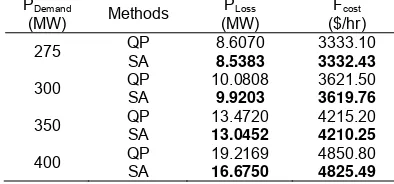
The optimal scheduling of generators obtained by the proposed SA algorithm for three unit systems is shown in Table 3. The comparison of results between conventional QP method and the proposed SA method are shown in Table 4. The comparison of results shows that the proposed SA algorithm is better than conventional QP method for each loading and it is very reliable in the aspect of solution quality.
Table 2. Economic dispatch for 3-generating units using QP method
PDemand
(MW)
P1
(MW)
P2
(MW)
P3
(MW)
PLoss
(MW)
Fcost
($/hr)
275 193.8232 74.7838 15.0000 8.6070 3333.10
300 207.6799 87.4010 15.0000 10.0808 3621.50
350 235.5798 112.8921 15.0000 13.4720 4215.20 400 250.0000 150.0000 19.2169 19.2169 4850.80
Table 3. Economic dispatch for 3-generating units using the proposed SA
PDemand
(MW)
P1
(MW)
P2
(MW)
P3
(MW)
PLoss
(MW)
Fcost
($/hr)
275 193.6474 74.8906 15.0002 8.5383 3332.43
300 207.6336 87.2867 15.0000 9.9203 3619.76
350 235.7958 112.2489 15.0006 13.0452 4210.25 400 249.9998 150.0000 16.6752 16.6750 4825.49
Table 4. Comparison of results between QP and the proposed SA for 3-generating units
PDemand
(MW) Methods
PLoss
(MW)
Fcost
($/hr)
275 QP
SA
8.6070 8.5383
3333.10 3332.43
300 QP
SA
10.0808 9.9203
3621.50 3619.76
350 QP
SA
13.4720 13.0452
4215.20 4210.25
400 QP
SA
19.2169 16.6750
4850.80 4825.49
Case 2: 6-Generating Units
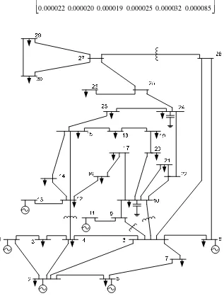
In this case, a standard of six-generating units (IEEE 30 bus test systems) is used to demonstrate how the work of the proposed approach, as shown in Figure 2. Characteristics of thermal units are given in Table 5, followed by coefficient matrix Bij losses.
The simulation results using the proposed SA algorithm are shown in Table 6 and Table 7 respectively for the load variation of 700 MW and 800 MW. The simulation results show that the generation outputs of each unit obtained were smaller than those of the genetic algorithm (GA), which is taken from [22]. Further, as a result, there was some reduction of the total generation cost and transmission losses.
Table 5. Generating unit capacity and coefficients
Unit min
i P
(MW) max
i P
(MW)
ai
($/MW2
) bi
($/MW)
ci
($) 1 10 125 0.0033870 0.856440 16.817750 2 10 150 0.0023500 1.025760 10.029450 3 35 225 0.0006230 0.897700 23.333280 4 35 210 0.0007880 0.851234 27.634000 5 130 325 0.0004690 0.807285 36.856880 6 125 315 0.0003998 0.850454 30.147980
000085 . 0 000032 . 0 000025 . 0 000019 . 0 000020 0 000022 . 0 000032 . 0 000069 . 0 000030 . 0 000024 . 0 000015 0 000026 . 0 000025 . 0 000030 . 0 000071 . 0 000017 . 0 000016 0 000019 . 0 000019 . 0 000024 . 0 000017 . 0 000065 . 0 000013 0 000015 . 0 000020 . 0 000015 . 0 000016 . 0 000013 . 0 000060 0 000017 . 0 000022 . 0 000026 . 0 000019 . 0 000015 . 0 000017 0 000140 . 0 . . . . . . Bij
Figure 2. IEEE 30-bus 6-generator test systems
Table 6. Economic dispatch for 6-generating units (PD = 700 MW)
Unit Output GA [22] SA
P1 (MW) 27.3010 26.7391 P2 (MW) 15.6124 12.2597 P3 (MW) 120.3109 126.3482 P4 (MW) 116.7756 117.6017 P5 (MW) 226.8377 230.3174 P6 (MW) 212.4050 205.9579 Total power output (MW) 719.2426 719.2241 Total generation cost
($/hr) 820.4200 820.3707
Table 7. Economic dispatch for 6-generating units (PD = 800 MW)
Unit Output GA [22] SA
P1 (MW) 32.6737 32.5980 P2 (MW) 15.8161 14.5035 P3 (MW) 141.6623 141.5182 P4 (MW) 131.3117 136.0152 P5 (MW) 252.3711 257.6949 P6 (MW) 251.5507 243.0010 Total power output (MW) 825.3855 825.3309 Total generation cost
($/hr) 931.1060 931.0322
Power losses (MW) 25.3855 25.3309
4. Conclusion
In this paper, an efficient simulated annealing (SA) algorithm with a single decision variable has been successfully introduced to obtain the optimum solution of economic load dispatch problem. The proposed SA method has been tested on two test cases consisting of 3-generating units and 6-3-generating units systems and the results are compared to those of the conventional quadratic programming method and the GA method. Test results have shown that the proposed method can provide better solution than above mentioned methods.
References
[1] Wood A.J, Wollenberg B.F. Power Generation, Operation, and Control. New York: John Wiley and Sons, 1984.
[2] Park J. B, Lee K. S, Shin J. R, Lee K. Y. A Particle Swarm Optimization for Economic Dispatch with Non-Smooth Cost Functions. IEEE Transactions on Power Systems. 2005; 20(1): 34-42.
[3] Liang Z. X, Glover J. D. A Zoom Feature for a Dynamic Programming Solution to Economic Dispatch Including Transmission Losses. IEEETransactions on Power Systems. 1992; 7(2): 544-550.
[4] Lee K.Y, Sode-Yome A, Park J. H. Adaptive Hopfield Neural Network for Economic Load Dispatch.
IEEE Transactions on Power Systems. 1998; 13(2): 519-526.
[5] Yalcinoz T, Short M. J. Neural Networks Approach for Solving Economic Dispatch Problem with Transmission Capacity Constraints. IEEETransactions on Power Systems. 1998; 13: 307-313. [6] Park J.H, Kim Y.S, Eom I.K, Lee K.Y. Economic Load Dispatch for Piecewise Quadratic Cost
Function Using Hopfield Neural Network. IEEETransactions on Power Systems. 1993; 8(3): 1030-1038.
[7] Yang H. T, Yang P. C, Huang C. L. Evolutionary Programming Based Economic Dispatch for Units with Non-Smooth Fuel Cost Functions. IEEE Transactions on Power Systems. 1996; 11(1): 112-118. [8] Andi Muhammad Ilyas, Nasir Rahman M. Economic Dispatch Thermal Generator Using Modified
Improved Particle Swarm Optimization. TELKOMNIKA. 2012; 10(3): 459-470.
[9] Youssef H. K. El-Naggar K. M. Genetic Based Algorithm for Security Constrained Power System Economic Dispatch. Electric PowerSystems Research. 2000; 53: 47-51.
[10] Orero S.O. and Irving M.R. Economic Dispatch of Generators with Prohibited Operating Zones: A Genetic Algorithm Approach. IEEE Proc. Gen.Transm. Distrib. 1996; 143(6): 529-534.
[11] Mithun M. B, Maheswarapu S. A Hybrid Genetic Algorithm Approach for Optimal Power Flow.
TELKOMNIKA. 2011; 9(1): 209-214.
[12] Nasimul Nomana, Hitoshi Iba. Differential Evolution for Economic Load Dispatch Problems. Electric
Power Systems Research. 2008; 78: 1322-1331.
[13] Lin W. M, Cheng F. S, Tsay M. T. An Improved Tabu Search for Economic Dispatch with Multiple Minima. IEEE Transactions on PowerSystems. 2002; 17(1): 108-112.
[14] Ismail Musirin, Nurhazima Faezan Ismail, Mohd. Rozely Kalil. Ant Colony Optimization (ACO)
Technique in Economic Power Dispatch Problems. Proceedings of the International Multiconference
of Engineers and Computer Scientists. Hong Kong. 2008; Vol. II IMECS 2008: 19-21.
[15] Abido M. A. Simulated Annealing Based Approach to PSS and FACTS Based Stabilizer Design.
Electric Power and Energy Systems. 2000; 22: 247-258.
[16] Sasikala J, Ramaswamy M. Optimal Based Economic Emission Dispatch Using Simulated Annealing. International Journal of Computer Applications. 2010; 1 (10): 55-63.
[17] Danaraj R.M.S, Gajendran F. Quadratic Programming Solution to Emission and Economic Dispatch Problems. Journal of the Institution of Engineers (India). pt EL., 2005; 86: 129-132.
[19] Kirkpatrick S, Gelatt Jr. C. D, Vecchi M. P. Optimization by Simulated Annealing. Science. 1983; 220: 671–680.
[20] Aarts E, Korst J. Simulated Annealing and Boltzmann Machines: A Stochastic Approach to Combinatorial Optimization and Neural Computing. New York. Wiley. 1989.
[21] Vanitha M, Tanushkodi K. Solution to Economic Dispatch Problem by Differential Evolution Algorithm Considering Linear Equality and Inequality Constrains. International Journal of Research and
Reviews in Electrical and Computer Engineering. 2011; 1(1): 21-26.
[22] Attia A. El-Fergany. Solution of Economic Load Dispatch Problem with Smooth and Non-Smooth Fuel Cost Functions Including Line Losses Using Genetic Algorithm. International Journal of

![Table 7. Economic dispatch for 6-generating units (P D = 800 MW) Unit Output GA [22] SA](https://thumb-ap.123doks.com/thumbv2/123dok/238019.502412/9.595.179.413.106.213/table-economic-dispatch-generating-units-mw-unit-output.webp)
