Energy-efficient Routing Model Based on Vector Field
Theory for Large-scale Wireless Sensor Networks
Ming Li1,2,a*, Huanyan Qian1,b, Min Xu3,c 1
School of Computer Science and Technology, Nanjing University of Science and Technology, Nanjing, 210094, China
2
School of Business, Hohai University, Nanjing, 211100, China
3Department of Accounting & Information Systems, California State University Northridge, Northridge, CA 91330-8372, USA
e-mail: [email protected]a, [email protected]b, [email protected]c
Abstract
Routing design is a key issue for large-scale wireless sensor networks (WSNs). Energy consumption associated with allocated resources should be considered. This paper proposes the integration of an energy-efficient model, which is based on vector field theory, in large-scale WSNs. Source nodes in WSNs have the characteristics of source points in a vector field, whereas sink nodes could be characterized as gathering points. Our scheme demonstrates that we can solve a set of partial differential equations in electrostatic theory to determine the routes that result in energy efficiency. Thus, the routing problem in WSN for energy efficiency becomes a typical PDE solution. Our simulation results show significant improvement in energy consumption. Compared with the traditional shortest path approach, the proposed model shows considerable improvement in the lifetime of the network.
Keywords: energy efficient, routing model, vector field theory, wireless sensor network
Copyright © 2015 Universitas Ahmad Dahlan. All rights reserved.
1. Introduction
Wireless sensor networks (WSNs) [1]–[3] consist of several hundreds to several thousands of sensors propagated in a geographical area. The sensors can communicate with each other through wireless links and often use radio frequency channels to communicate. The sensors measure specific metrics like, such as temperature, pressure, movements, or other physical values, in a periodic or non-periodic manner. However, the sensors utilize battery power, and efficient energy use of sensors is crucial to increase the lifetime of the network. Thus, determining optimal transmission paths from each sensor to the destination is important.
The routing problem in sensor networks has been studied by many researchers. S. Toumpis and L. Tassiulas first introduced electrostatic field theory into the WSN [4]. Their works focus on the sensor deployment problem in WSNs. The researchers abstracted the node optimal distribution problem into a charge distribution problem in the electrostatic field, thus providing an effective concept of building up the routing model for WSNs.
Mehdi Kalantari and Mark Shayman used electrostatic field theory to study ad hoc networks and verified the feasibility of analyzing work routing with the electrostatic field. On the basis of a previous work [7], they also employed vector analysis in the literature [8] and described the routing problem in WSNs with the differential equation in the electrostatic field. They derive the partial differential equation according to the properties of the electrostatic field, applied the equation to route WSNs, and employed the mathematical physics method to solve the energy routing problem of WSNs.
A previous work in the literature [10–12] adopted the theory analysis method of the Euler equation, which is based on the flow field to simulate the mobility of sensor nodes in WSNs to ensure balanced distribution of nodes, effective utilization of energy, and coverage rate of high networks. Alireza Salehan et al [13] modified the framework of the simulation of WSNs and simulated the communication process of the ad hoc network in a flow model. According to simulation results of the algorithms, such as DSDV, DSR, AODV, and TORA, the researchers verified the correctness of the flow model.
By integrating the descriptions in the previous works above, we determine that all the said problems can be transformed into definite solution problems of typical mathematical physics based on static charge movement in the electrostatic field or fluid particle movement in the flow field and the electrostatic field difference equations or Euler equations. In this paper, we analyze the features of the field in WSNs by using vector field theory to determine the effective energy route for WSNs.
2. WSN Model Based on Vector Field Theory 2.1. Introduction of Vector Field Theory Model
Considering that a WSN consists of N nodes, we assume that each node can communicate through wireless channels and the nodes are placed in a planar region called A. When events occur somewhere in the network, the closest node will trigger a message. Each node attempts to obtain the message in the sensor network and responds to the message of the neighboring node. Finally, all the messages are transmitted to the sink node. Considering the completeness of a model, we make the following assumptions:
A1: Every node carries limited energy, and the residue energy time is noted;
A2: In sensor networks, every geographic region that generates trigger events is accompanied by a given regional load density distribution law. The load density in
represents the load generated in
by a unit time. If we assume that the coordinate in
is (x,y), then we record that the load density in
is
( , )
x y
. The value ofw s
( )
reflects the load generated in place a a
A by unit time. That is to say, the rate generated by trigger events is as follows:( )
( , )
a
w s
x y d
(1)In the formula above,
w s
( )
is the integral in flat area a,d
is the differential unit in theplanar region including
;A3: The position of the node is fixed and knowable;
A4: When the node is deployed, each node in the network can arrive at the sink node through a multi-hop transmission sequence;
A5: To find the route, we provide a direction to each point in sensor networks, which points the next nearest node, and assume that it is a continuous function about
.On the basis of assumption A2, the rate of each sensor that generates a message can be derived according to its response trigger events within the region. Wi is used as the load of
sensor node i, which shows the rate of node i producing messages. If
t
i represents the region where the sensor node i is responsible for responding to trigger events, then Wi can be derivedby the area integral in
i
t
based on Formula (1). The value of Wi is the weight of node i. WeAt the same time, we assign a weight to the sink node using
w
0 to express the sinknode. We use Formula (2) to define the sink node
0 i 1
w
N
i
w
(2)Formula (2) should show that the rate of the sink node that receives the message is the total rate of all the source nodes that send messages to the sink node and the negative value indicates the role of the sink node.
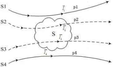
We define the path as a directing curve derived from the initial node to the sink node. Thus, N corresponding paths exist in the sensor network containing N source nodes. We use
i
p
to express the path of sensor node i. The load of each path is the rate of the original nodeproducing messages in the path. Thus, the weight of path
p
i isw
i.According to the abstract path set from each sensor node to the sink nod, we define a vector field on region A as a load vector field, denoted by
D
, which represents the message speed distribution field in sensor networks and the directions of all the points to the sink node. Given any point
in region A, we select the minimal region unit area a in
. When area S of a infinitely tends to be 0, we can derive the load vector of every point, as shown in Formula (3)0
1
( )
lim
i
i i S
p S
D
w l
S
(3)
In the formula above,
l
i is the unit tangent of pathp
i in region S, which directs the destination node along the path. Figure 1 illustrates the above definition. On the basis of thedescription of Hypothesis 5, all the paths through S will have the same unit tangent
l
i whenS
tends to be zero. Thus, result
D
( )
added by the vectors in Equation (3) will have the samedirection. In other words,
D
( )
is the sum of all the path loads through region S, and it reflectsthe actual communication activity of place
in the sensor network, which is the messagetransfer condition in
. On the basis of field theory, load vectorD
can also be called the load density.Mathematically, if the number of sensors is limited, then the value of
D
may be zero only when the set is empty. We can divide region S into several rectangular areas using the vertical and horizontal grid line. When these rectangular elements are sufficiently small, we can treatD
as a continuous variable for processing.We define the integral when load vector field
D
points to the direction of the curve as follows:D dn
(4)It is the load flux when
D
passes through the curve
, which denotes the message volume per unit time through the curve
.If the defined
in Equation (4) is a closed curve, then the definedD
in Equation (3) must meet the following equation:
D dn
w
(5)In the previous formula,
is a closed curve.dn
is a normal differential vector of each point on the closed curve, and
w
is the load sum of nodes within the closed area. In the electrostatic field, Gauss’s law exhibits a similar form, which shows that the electric flux through a closed curve is proportional to the amount of charges surrounded by a closed curve. For the steady incompressible fluid in the flow field, the above formula also shows the unique physical significance. The flow produced by a source within fluid blocks in a unit time is equal to the fluid quality from the surface of the fluid blocks in the same time period.In sensor networks, if a message is transferred from the node outside the closed curve to a node inside it, then we can say that the message enters the closed area. Otherwise, we can assume that the message exits the closed area. According to the definition above, Equation (5) indicates that the generated message amount in the unit time of a closed region is the sum of the real-time message transmission rates between internal nodes.
We define characteristic function
, which shows that the message reaches the planar region, and its value is about the position function. If
( )
( , )
x y
, then, except for the sink node, the value of
( )
is that of
( )
.0 0
( )
( )
w
(
)
(6)On the basis of the definition of
stated above, Equation (5) can be rewritten into the differential equation according to the formula of Green.( )
( )
D
(7)
In the formula above,
is defined asi
j
x
y
(8)
In the formula, x and y represent the horizontal and vertical axes in the Descartes Cartesian rectangular coordinate system, respectively.
i
and
j
denote the unit normal vectors along axial coordinate x, y.(
)
0,
n
D
the edge of the area A
D
(9)
In the formula above, A is the area set in the sensor network.
D
n( )
shows the scalaralong the boundary of region A by
D
. The first equation of Equation (9) explains that all the message flows produced in the network will finally point to the sink node. The second equation derives from the fact that no message flow comes out of the sensor network area boundary.2.2. Establishing the Load Vector Field
On the basis of the vector field theory model, which is illustrated in the former section, combined with electrostatic field theory and fluid mechanics theory, we determine that the load vector field of the sensor is similar to the electrostatic field in theory of electromagnetic field and the flow field in fluid mechanics. Similar to the electric field lines in the electrostatic field and the streamline field lines in the flow field, we define the concept of the load line in sensor networks. Load line is an instantaneous smooth curve in the load vector field where the transmission direction of the message unit coincides with its tangent direction. Obviously, the load line is similar to the electric field line and streamlines field line, except for some special points that neither turn nor intersect.
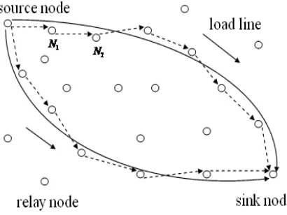
By establishing the load vector field and defining the concept of load line, we can determine the route from the source node to the destination node according to Formula (5). The load line can be approximately considered the space–transfer curve of the message unit in a time interval. By identifying optimal solution
D
that satisfies the model, we can describe our load vector field according to the gradient function and determine the route of the WSN based on the load line.Figure 2. Sample of load line routing
3. WSN Energy Efficiency Routing Based on a Stable Field Model and Solution
The routing mechanism in the traditional network usually selects the path with the minimum cost between the source node and the sink node. In fact, we should consider the balance of the whole network load and the network survival time in selecting the network routing because of the limited node energy consumption. The core problem of the energy efficiency routing is selecting the route according to the energy consumption and the residual energy of the nodes in the path.
In establishing the load vector field, we define a space vector for each point in the space and also set up an energy field for each point in the space, which is a residual energy distribution function on point
.0
node i
1
( , )
lim
i( )
S
S
w
t
e t
S
(10)In the previous formula,
e
i( )
t
represents the residual energy of the sensor node i attime t. Evidently,
w
( , )
t
will probably be zero when the energy set is empty only in the place of
.3.1. Energy Routing Under a Stable Field Model
We assume that the initial energy of the WSNs is unified allocated, i.e.,
w
( , 0)
c
(cis a constant). To determine the energy efficiency route, we must maximize D( )
in each point
of
under the communication condition of the sensor network. D( ) represents the instantaneous message transmission rate in
of the sensor network. Thus, the attenuation ofenergy per unit time in
can be approximately proportional toD( ) .A unified D is made as far as possible to determine the energy efficiency routing evenly spreads the transmission of messages in the network. Hence, we can avoid some nodes in the network that are not fully utilized and overused.
A unified load distribution can be expressed according to the following minimum cost function.
2
( )
avA
J D
D
D
ds
(11)In the formula above,
D
av
is a mean value of vector field
D
in the set of A. It can be defined simply as
1
av
A
D
Dds
A
(12)
2
( )
( )
0
av
A
n
Minimize J D
D
D
ds
D
D
the edge of A
subj ect t o
:
,
(13)
The following lemmas provide key ideas in the optimization problem for Equation (13).
Lemma 1: If
D
represents the optimal solution of Equation (14), then it must satisfy the following equation:
D
0
(14)
In the equation above, is a 2D direction vector operator. In vector field
x y
F F F, we define this operation with the formula
y x
F
F
F
k
y
x
(15)where
is a unit complex vector, which is composed of
i
and
j
, i.e.,
i
j
. On the basis of the above lemma, we can write a set of spatial difference equations for optimal solutionD
.D
,
D
0
(16)The above equations are similar to the Maxwell equations of electrostatic field theory. In spatial difference equation theory, we verified the boundary conditions of the above equations, which can be given particularly through
D
. In the model of mathematical field theory, thevector field that satisfies
D
0
is also called a conservative vector field, which can be expressed as the gradient of the scalar field, i.e.,D
U
(17)
U is a potential function, and it can be drawn according to directional derivatives, which we call the scalar function. Equation (16) can be simplified to
2U
.Operator
2is defined as2 2 2 2 2
x
y
(18)The boundary condition of
D
implies that the tangent direction of the gradient of U along the boundary curve is always 0, which has the following form using the formula:
ˆ
( )
( )
0,
U
n
the edge of A
(19)
ˆ( )
n
expresses the unit tangent vector of point
along the direction of the boundary curve.3.2. Definite Conditions under the Model of the Stable Field
In Section 4.1, we presented key ideas about the load cost function in a WSN under an ideal state and the optimum solution of the differential equations. In this section, we summarize the load vector field property of the field model that was unified and distributed by the initial energy of the sensor node.
D 0
D
(20)
The above differential equations from the microscopic point of view explain the active and irrotational characteristics of the load vector. D 0. Thus, we can find a scalar function U to establishD U. We define U as the load potential in the vector field. The change rate of
the load potential in any direction of
l
i is equal to the numerical value of the load vector in thisdirection (
l
i is the unit vector in the direction).D l i
u
D l
l
(21)
Thus, along direction
l
i, the increasing amount of the load potential is as follows:D
l i
du D dl d l (22)
The load potential difference between two points, namely, arbitrary P and Q, along the
direction
l
i is as follows:D Q
Q P i P
u u u d l
(23)Equation (23) reflects the cost paid by the vector field when the message unit moves from point Q to point P.
On the basis of the differential equation sets, the differential equations that satisfy the load potential of a load vector field in sensor networks can be derived. We integrate
D
U
into the second equation of Formula (20), thereby forming 2
D
(
U
)
U
where 2U
is a Poisson’s equation that is correct for any point of the vector field in the model. In the region where the transmission of the message unit does not occur, the above formula is transformed into Laplace’s equation.2
0
U
(24)intensity and the load potential on both sides of the specific interface when message units are being transmitted.
4. Simulation and Analysis 4.1. Routing
A total of 300 sensor network nodes are randomly distributed in a plane area of 500*500. Assume all nodes belong to the routing node except the sink node and the source node. In this case, the load potential of any point in the load vector field is the superposition of potentials of all source nodes in the point. Figure 3 simulates the single-source node and the single-sink node; the source node is in the upper left corner in the scene, whereas the sink node is in the lower right corner.
Figure 3. Single-source single-sink scene: velocity vector and potential field line (left), potential field line and streamlin. It is the load flux e (right)
Paper also explores the simulation of the multi-source node and multi-sink node scene (Fig. 4) where the source nodes and sink nodes are marked in the figure. The figure indicates the load vector field obtained according to the superposition principle.
Figure 4. Multi-source, multi-sink scene: velocity vector and potential field line (the left picture), potential line and streamline (the right picture)
-500 0 500
-500 -400 -300 -200 -100 0 100 200 300 400 500
-500 0 500
-500 -400 -300 -200 -100 0 100 200 300 400 500
-500 0 500
-500 0 500
sink1
source1
source2
source3
source4 sink2
-500 0 500
-500 0 500
sink1
source1
source2
source3
4.2.Result Analysis and Performance Comparison
The paper uses the MATLAB platform tool to carry out routing performance analysis and chooses four indices, namely, network delay, throughput, successful delivery rate, and energy consumption, to evaluate the performance of a routing protocol.
The paper compares vector field routing (VF), the routing protocol proposed with many classical routing protocols, such as energy-efficient ant-based routing protocol (EEABR), sensor-driven and cost-aware ant routing (SC), flooded forward ant routing (AF), flooded piggybacked ant routing (FP), basic ant-based routing (BABR), ad hoc on-demand distance vector (AODV), and adaptive spanning tree (MCBR-AST). Table 1 provides the simulation parameters.
Table 1. Simulation parameters
Parameter Value
Routing It is the load flux protocol VF, EEABR, SC, FF, FP, BABR, AODV, MCBR-AST Number of nodes 300
Maximum hop count 30
Data transmission Constant bit rate (CBR) Transmission rate 500 kbps
Simulation time 100 s Node energy 80 J.
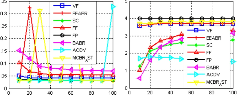
The following performance analysis chooses FF, SC, and AODV for the comparison. In the left picture in Figure 5, the network delay of VF is significantly lower than that of FF but slightly higher than those of SC and AODV. VF contains multiple paths, including the shortest path, the path from the source node to the destination node, and the average hop count of all the paths, which is higher than that of the shortest path. Thus, the network delay is slightly higher. The simulation result indicates that the network delays of VF and AODV are 0.0421 and 0.036 s, respectively. The delay of FV is higher by 25% or so.
Figure 5. Network delay (left picture) and network throughput (right picture)
The right picture in Figure 5 determines that the throughput of FV is higher than those of the three routing protocols because VF can transmit data through multiple paths simultaneously, but AODV has only one transmission path. The simulation result shows that the number of data packets sent in AODV reaches 1024 the number in VF is 3321, which is approximately triple that of the former. Moreover, the figure indicates that the throughput of SC and FF increases with time, whereas VF does not exhibit this phenomenon but remains stable at 3.8 or so.
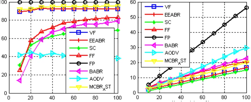
Conversely, in the other three protocols, the index is low at the beginning of the simulation. For SC and FF, the successful delivery rate increases, whereas the index decreases for AODV. The index of VF is significantly higher than those of the three other protocols (the highest point is roughly 50% higher than the lowest point).
Figure 6. Successful delivery rate (left picture) and network energy consumption (right figure)
The right picture in Figure 6 demonstrates that the energy consumption of the network for all protocols increases in the simulation process. AODV has the highest energy consumption, whereas SC exhibits the smallest energy consumption. Moreover, the slope of AODV curve is higher than that of the VF curve, thereby indicating the former consumes more energy with time.
5. Conclusion
In this paper, from the perspective of the conservation of node power consumption, we find a routing mechanism for WSNs for high-efficiency energy use of the entire network. We establish a WSN model of the vector field according to the characteristics of transferring packets in the WSNs. We introduce a WSN model based on vector field theory. The process of transferring message packets produced by the source sensor node to the sink node through a certain path defines a load vector for every position in the network. We attem It is the load flux pt to ensure the optimal solution of the network by establishing the load vector field to determine the ideal routing of the wire. It is the load flux WSN.
Evidently, some aspects of this paper need to be improved. We simulate only the vector field in a plane area in the MATLAB simulation of the typical vector field. For the 3D space model, describing the load vector field is feasible. At the same time, our simulations were conducted for only the unified situation under the initial state. The initial state is not a unified situation. Thus, the choice of routing is closely related with time. We can integrate a mathematical physics equation that is similar to the diffusion process or the transfer process for modeling. This option is a future research direction and improvement of this paper.
References
[1] Pantazis, Nikolaos A, Nikolidakis, Stefanos A, Vergados, Dimitrios D. Energy-Efficient Routing Protocols in Wireless Sensor Networks: A Survey. IEEE Communications Surveys & Tutorials. 2013; 15(2): 551-591
[3] Hongwei Du; Weili Wu; Qiang Ye; Deying Li; Wonjun Lee; Xuepeng Xu. CDS-Based Virtual Backbone Construction with Guaranteed Routing Cost in Wireless Sensor Networks. IEEE Transactions on Parallel and Distributed Systems. 2013; 24(4): 652-661
[4] Toumpis S, Tassiulas L. Packetostatics: Deployment of Massively Dense Sensor Networks as an Electrostatics Problem. Proceedings IEEE 24th Annual Joint Conference of the IEEE Computer and Communications Societies. 2005; V4: 2290-2301
[5] Toumpis S, Gupta GA. Optimal Placement of Nodes in Large Sensor Networks under a General Physical Layer Model. 2005 Second Annual IEEE Communications Society Conference on Sensor and Ad Hoc Communications and Networks. 2005; 275-283
[6] Choi Y, Syed I, Kim H. Event Information Based Optimal Sensor Deployment for Large-Scale Wireless Sensor Networks. IEICE Transactions on Communications. 2012; E95B(9): 2944-2947 [7] Zhao Wei, Tang Zhenmin, Yang Yuwang, Yu Jiming, Wang Lei. Routing in Wireless Sensor Network
Based on Field Theory. Journal of Computational Information Systems. 2012; 8(5): 1-8
[8] Nikolidakis, Stefanos, Kandris, Dionisis, Vergados, Dimitrios, Douligeris, Christos. Energy Efficient Routing in Wireless Sensor Networks Through Balanced Clustering. Algorithms. 2013; 6(1): 29-42 [9] Peng J, Chen XH, Liu T. A Flow-Partitioned Unequal Clustering Routing Algorithm for Wireless
Sensor Networks. International Journal of Distributed Sensor Networks. 2014; 57(6): 1-12
[10] Khawam K, Samhat AE, Ibrahim M, Kelif JM. Fluid Model for Wireless Adhoc Networks. 2007 IEEE 18th International Symposium on Personal, Indoor and Mobile Radio Communications. 2007; 1-5 [11] Venkatsampath Raja Gogineni, Kalyan Matcha, Raghava Rao K. Real Time Domestic Power
Consumption Monitoring using Wireless Sensor Networks. International Journal of Electrical and Computer Engineering. 2015; 5(4): 685-694
[12] Daroczy L, Jarmai K. From a quasi-static fluid-based evolutionary topology optimization to a generalization of BESO. Engineering Optimization. 2015; 47(5): 689-705
[13] Salehan A, Robatmili M, Abrishami M, Movaghar A. A Comparison of Various Routing Protocols in Mobile Ad-hoc Networks (MANETs) with the Use of Fluid Flow Simulation Method. 2008 The Fourth International Conference on Wireless and Mobile Communications. 2008; 260-267
[14] Zhen Ni, Qianmu Li, Tao, Li, Yong Qi. A WSN Nodes Access Mechanism and Directed Diffusion in Emergency Circumstances. Journal of Digital Information Management. 2014; 12(4): 235-245
[15] Ayadi M, Affonso RC, Cheutet V, Masmoudi F, Riviere A, Haddar M. Conceptual Model gor Management of Digital Factory Simulation Information. International Journal of Simulation Modelling.
2013; 12(2): 107-119