DOI: 10.12928/TELKOMNIKA.v12i4.531 977
Multi-objective Optimization Based on Improved
Differential Evolution Algorithm
Shuqiang Wang*1, Jianli Ma2
1
School of Information and electrical engineering, Hebei University of Engineering, Handan 056038, Hebei, China
2
Suburban water and power supply management office of Handan City, Handan 056001, Hebei, China *Corresponding author, e-mail: [email protected]
Abstract
On the basis of the fundamental differential evolution (DE), this paper puts forward several improved DE algorithms to find a balance between global and local search and get optimal solutions through rapid convergence. Meanwhile, a random mutation mechanism is adopted to process individuals that show stagnation behaviour. After that, a series of frequently-used benchmark test functions are used to test the performance of the fundamental and improved DE algorithms. After a comparative analysis of several algorithms, the paper realizes its desired effects by applying them to the calculation of single and multiple objective functions.
Keywords: differential evolution, effect of parameters, numerical experiment, multi-objective optimization
1. Introduction
In the scientific research and engineering design, many specific problems can be summarized as the problems of parameter optimization. However, in practice, these optimization problems usually have multiple design objectives, which contract with and restrict each other [1]. The performance optimization of one problem usually leads to the performance degradation of at least one of the other problems, which indicates that it is difficult to make many objectives to reach optimization simultaneously. Therefore, the research of multi-objective optimization algorithm has become a research hospot in current science and engineering design [2]. Evolutionary algorithm is the general term of heuristic research and optimization algorithms inspired and developed from natural biology and system and to solve multi-objective optimization problems with evolutionary algorithm has been widely used [3].
As an important part of evolutionary algorithm, differential evolution has been widely used in solving optimization problems because it has simple theory, simple operation and strong robustness [4]. The basic principle of differential evolution is to disturb a certain individual in the group and search the search space; however, it is too random in choosing the individuals generating differences and it is easy to cause algorithm prematurity or long-time optimization so as to make it unable to obtain global optimization solution [5]. Besides, when settling multi-objective optimization problems, differential evolution is affected by its own limitations, making the selection of mutation strategy and the setting of parameter values seriously restrict the performance of the algorithm [6].
2. DE Algorithm
2.1 Basic Ideas of DE Algorithm
DE algorithm is an evolutionary algorithm based on real-number encoding to optimize the minimum value of functions. The concept was put forward on the basis of population differences when scholars tried to solve the Chebyshev polynomials. Its overall structure is analogous to that of genetic algorithms. The two both have the same operations such as mutation, crossover, and selection [7]. But there are still some differences. Here are the basic ideas of DE algorithm: the mutation between parent individuals gives rise to mutant individuals; crossover operation between parent individuals and mutant individuals is applied according to certain probability to generate test individuals; greedy selection between parent individuals and test individuals is carried out in accordance with the degree of fitness; the better ones are kept to realize the evolution of the population [8].
2.1.1 Mutation Operation
x x x x are three individuals randomly selected from the population;
1
mutation operator that lies between [0.5,1]. So we can obtain mutant individual t i
individual xit in line with the following principle:
In the expression, rand[0,1]is a random number between [0,1]; CR, the crossover operator, is a constant at [0,1]; the bigger CR is, the more likely crossover occurs; j_randis an
integer randomly chosen between [1,D], which guarantees that for test individual t i
u , at least
one element must be obtained from mutant individual t i
v . The mutation and crossover operations are both called reproduction [9].
2.1.3 Selection
DE algorithm adopts the “greedy” selection strategy, which means selecting one that has the best fitness value from parent individual t
i
x and test individual t i
u as the individual of the next generation. The selection is described as:
1 ( ) ( )
t t t
t i i i
i t
i
x if fitness x fitness u x
u otherwise
Where fitness, the objective function to be optimized, is regarded to be the fitness function. Unless stated, the fitness function in the paper is an objective function with a minimal value[10].
2.2 Calculation Process of DEAlgorithm
From the principles of fundamental DE algorithm mentioned above, we can understand the calculation process of DE algorithm as follows:
(1) Parameter initialization: NP: population size; F: scale factor; D: spatial dimension of mutation operator; evolution generationt0.
(2) Random initialization of the initial population ( ) { 1, 2, , }
(3) Individual evaluation: calculate the fitness value of each individual.
(4) Mutation operation: mutation operation is applied to each individual in accordance with Expression (1) to work out mutant individual vit.
(5) Crossover operation: crossover operation is applied to each individual in accordance with Expression (2) to work out test individual uit.
(6) Selection: select one from parent individual xit and test individual t i
u as the individual of the next generation in accordance with Expression (3).
(7) Test termination: the next generation of population generated from the above process is
1 1 1
the maximum evolution generation or meets the criteria of errors, merge and output xbestt 1
as the optimal solution; otherwise, make t t 1and return to step (3).
2.3 Parameter Selection of DEAlgorithm 2.3.1 Selection of Population Size NP
In view of computation complexity, the larger the population size is, the greater the likelihood of global optimal solution becomes. But it also needs more calculation amount and time. Nonetheless, the quality of the optimal solution does not simply gets better as the population size expands. Sometimes, it’s the other way round. The accuracy of solutions even declines after population size NP increases to a certain number. This is because a larger population size reduces the rate of convergence, though it can keep the variety of population. Variety and the rate of convergence must be kept in balance. Hence, the accuracy will decrease if the population size gets larger but the maximum evolution generation remains unchanged. The larger the population size is, the greater the variety is. Therefore, a larger population size is needed to expand variety and prevent premature convergence of a population [11].
According to our previous research results, the appropriate population size for simple low-dimensional problems should lie between 15 and 35 in the case of given maximum evolution generation. In the same circumstance, the population size that maintains between 15 and 50 helps keep a good balance between variety and the rate of convergence [12].
2.3.2 Selection of Scale Factor F
Let us test the performance of scale factor F. Set the population size at 15. Make sure the crossover operator and the maximum evolution generation stay unchanged.
Based on the test on scale factor F of the banana function, we know that in the case of the same initial population, the results of every 30 times of running vary greatly from each other when F0.7, and we can get better local optimization and faster rate of convergence at the expense of lower success rate of optimization and longer running time; when F0.7, there are no significant differences between the results of every 30 times of running, and we can get better global optimization, shorter running time, and faster rate of convergence.
convergence. Hence, the value of F should be neither too big nor smaller than a specific value[13]. This explains why the algorithm has good effects when F[0.7,1].
2.3.3 Selection of Crossover Operator CR
To test the effect of crossover operator on algorithm performance, we make the scale factor F0.9 and set population size at 20. Make the crossover operator lie between 0 and 1. Set the interval at 0.1. Let the maximum evolution generation remain the same.
The test shows the banana function can change CR. Thus, in the case of the same initial population, the results of every 30 times of running vary greatly from each other when
0.3
CR , and we can get better local optimization at the expense of slower rate of convergence, lower success rate of optimization and longer running time; when CR0.3, there are no significant differences between the results of every 30 times of running, and we can get better global optimization; but when 0.3CR0.6, we get slower rate of convergence and longer running time; when CR0.6, we get faster rate of convergence and shorter running time[14].
3. Simulation Testing of Five Improved DEAlgorithms 3.1 Five Improved DEAlgorithms
The fundamental DE algorithm can be described as: DE/rand/1/bin. “bin” means crossover operation. DE/x/y/z is used to differentiate the other DE deformations. xdefines whether the variant vector is “random” or “optimal”, ydenotes the number of residual vectors used, and zstands for the method of crossover operation. Below are the DE deformations if we only consider the selection modes of base points and the number of difference vectors:
DE/rand/1
(4) Multimodal function
2 2 0.25 2 2 0.1 2
1 2 1 2 1 2
( ) (( ) ) ((sin(50 ( ) ) ) 1) 5.12 , 5.12
f x x x x x x x
(7)
The minimum value here is 0 and there is an infinite local minimum. Below are the graphs of the above four test functions:
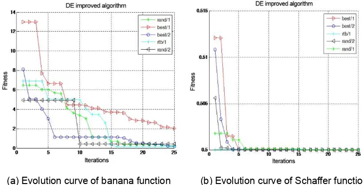
(a) Banana function (b) Schaffer function
(c) Bohachevsky function (d) Multimodal function
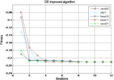
(c) Evolution curve of Bohachevsky function (d) Evolution curve of multimodal function
Figure 2. Evolution curves offour benchmark test functions
3.3 Test Results
Test the five algorithms using the test functions introduced in 3.2. NP15, F0.9, 0.9
CR , and the maximum evolution generation is 200. Average the results of the 30 times of running and we can get the evolution curves shown as in Figure 2.
According to the results and evolution curves of the above test functions, in the case of the same initial population, there are no significant changes in the results of every 30 times of running. Besides, the five improved algorithms can optimize functions well and thus yield very good results. For different functions, the rate of convergence varies, so does the efficiency of finding optimal solutions. The five algorithms have similar optimal performance, but some algorithms have longer running time and some functions have better optimization.
4. Application of DEAlgorithm in Multi-objective Optimization
Based on the previous description, DE algorithm is of great importance in solving complicated optimization problems. In the next part, we use DE algorithm to solve single- and multiple-objective optimization problems with equality constraints or inequality constraints.
4.1Single-objective Optimization Problem
The standard form of single-objective optimization is generally expressed as:
min f x x x( ,1 2, 3,,xn)
s.tg x x xi( ,1 2, 3,,xn)0 i1, 2,3,,m
h x x xj( ,1 2, 3,,xn)0 j1, 2, 3,,l (8)
ai xi bi
In the expression, penalty function D x( ) is a continuous function that meets
The structure of penalty function depends on the exterior point method:
3
For an objective function, we can first find its minima and then use DE algorithm so as to find the maxima of the function. The conversion method is the fitness function below:
3 way, the maximization of an unconstrained problem is converted into a minimization problem.
4.2 Multi-objective Optimization Problem
Under normal conditions, the multiple objective function is expressed as:
1 1 2 2
From the evolution curves and running results, we know that all the five improved DE algorithms can find their corresponding optimal solutions in the 30 times of running. The algorithms remain quite stable. However, they have different rate of convergence and running time.
5 Conclusion
This paper describes the design ideas of DE algorithm and further improves the parameters of the algorithm. After that, it compares the results of the numerical experiment and then analyzes the performance of the improved DE algorithms, thus providing the basis for the application of the algorithms. In the end, the paper adopts the penalty function method and the weighted strategy to deal with the constraint conditions of multiple-objective optimization problems and uses the improved DE algorithms to solve constrained optimization problems. Thereby, it helps expand the application areasof the DE algorithm.
References
[1] Matthias Ehrgott, Jonas Ide, Anita Schöbel. Minmax robustness for multi-objective optimization problems. European Journal of Operational Research. 2014; 239(1): 17-31.
[2] Marko Kovačević, Miloš Madić, Miroslav Radovanović, Dejan Rančić.Software prototype for solving multi-objective machining optimization problems: Application in non-conventional machining processes. Expert Systems with Applications. 2014; 41(13):5657-5668.
[3] Jan Hettenhausen, Andrew Lewis, Timoleon Kipouros. A Web-based System for Visualisation-driven Interactive Multi-objective Optimisation. Procedia Computer Science. 2014; 29: 1915-1925.
[4] Banaja Mohanty, Sidhartha Panda, P.K. Hota. Differential evolution algorithm based automatic generation control for interconnected power systems with non-linearity. Alexandria Engineering Journal. 2014; 53(3): 537-552.
[5] Piotr Jędrzejowicz, Aleksander Skakovski. Island-based Differential Evolution Algorithm for the Discrete-continuous Scheduling with Continuous Resource Discretisation. Procedia Computer Science. 2014; 35: 111-117.
[6] Saber M. Elsayed, Ruhul A. Sarker, Daryl L. Essam. A self-adaptive combined strategies algorithm for constrained optimization using differential evolution. Applied Mathematics and Computation. 2014; 241(15): 267-282.
[7] Coello C A C. Evolutionary Multi-Objective Optimization A Historical View of the Field. IEEE Computational Intelligence Magazine. 2010; 1(1): 28-36.
[8] Laumanns M, Thiele L, Deb K, Zitzler E. Combining Convergence and Diversity in Evolutionary Multi-Objective Optimization. Evolutionary Computation. 2010; 10(3): 263-282.
[9] Deb K, Pratap A, Agarwal S, Meyarivan T. A Fast and Elitist Multi-objective Genetic Algorithm: NSGA-II. IEEE Transactions on Evolutionary Computation. 2009; 6(2): 182-197.
[10] Zitzler E, Deb K, Thiele L. Comparison of Multi-objective Evolutionary Algorithms: Empirical Results.
Evolutionary Computation. 2010; 8(2): 173-195.
[11] Knowles J, Corne D. Approximating the Nondominated Front Using the Pareto Archived Evolution Strategy. Evolutionary Computation. 2011; 8(2): 149-172.
[12] Coello C A C. Evolutionary Multi-Objective Optimization: Some Current Research Trends and Topics That Remain To Be Explored. Frontiers of Computer Science in China. 2009; 3(1): 18-30.
[13] Reyes-Sierra M, Coello C A C. Multi-Objective Particle Swarm Optimizers: A Survey of the State-of-the-art. International Journal of Computational Intelligence Research. 2006; 2(3): 287-308.