DOI: 10.12928/TELKOMNIKA.v14i3A.4390 208
Forecasting Range Volatility using Support Vector
Machines with Improved PSO Algorithms
Liyan Geng1, Yigang Liang*2, Zhanfu Zhang3, Xin Shi4
1,2
School of Economics and Management, Shijiazhuang Tiedao University, Shijiazhuang, Hebei, 050043, P. R. China
1
Institute of Quantitative & Technical Economics, Chinese Academy of Social Sciences, Beijing, 100732, P. R. China
3
Department of Electrical and Engineering, Sifang College, Shijiazhuang Tiedao University, Shijiazhuang, Hebei, 051132, P. R. China
4
Business School, Manchester Metropolitan University, Manchester, M15 6BH, UK
*Corresponding author, e-mail: [email protected], [email protected], [email protected], [email protected]
Abstract
Financial volatility forecasting is an important content in financial derivatives pricing, financial risk management, portfolio allocation. Support vector machines (SVM) has been successfully used in modeling and forecasting volatility. To enhance the volatility forecasting ability of SVM, this paper introduced three improved particle swarm optimization (IPSO) algorithms into SVM for forecasting range volatility. SVM was used to construct the volatility forecasting model. And, the three IPSO algorithms: stochastic inertia weight PSO (SIWPSO), time-varying acceleration coefficients PSO (TVACPSO) and two-order oscillating particle swarm optimization (TOOPSO) were applied to finding the optimal parameters in SVM, respectively. The accuracy of the proposed models in forecasting range volatility was demonstrated by using three stock indices in China stock market. The empirical results imply that compared to SVM with SIWPSO and TVACPSO algorithms, SVM with TOOPSO algorithm produces higher accuracy in forecasting range volatility and faster speed on searching for the optimal parameters of SVM.
Keywords: volatility forecasting, support vector machines, improved particle swarm optimization algorithm
Copyright © 2016 Universitas Ahmad Dahlan. All rights reserved.
1. Introduction
In financial field, volatility forecasting has always been one of the central issues to be explored. Many researchers tried to construct a variety of models to forecasting financial volatility. One of the most classic volatility models is the GARCH model in [1]. GARCH model is the generalized form of the ARCH model [2]. With the lagged conditional variance, GARCH model captures the time-varying conditional volatility well and provides acceptable forecasting performance.
With information science and computer technology developing, artificial intelligent prediction methods have been widely used in volatility forecasting and formed a new type of volatility forecasting models. The two representative models are artificial neural network (ANN) and support vector machines (SVM). With the advantages of strong learning and self-adaptive ability, ANN can accurately describe the nonlinearity of financial volatility and has shown good ability in volatility forecasting. Donaldson [3] applied ANN to GARCH model for forecasting volatility. Dadkhah [4] and Tae [5] directly forecasted stock return volatility by using ANN. Bildirici [6], Hajizadeh [7] and Kristjanpoller [8] combined ANN with GARCH-type models to forecasting volatility, respectively. These studies indicated that ANN improved the accuracy in volatility forecasting based on its data-driven nonparametric and nonlinear properties. Nevertheless, the application of ANN often suffers from problems, such as excessive learning, local minimal value, calamity data and so on. These problems have restricted the popularization and application of ANN.
classification, and regression forecasting with its excellent generation performance. [10-13] applied SVM to forecast financial volatility, respectively and achieved better forecasting accuracy than ANN and the traditional volatility forecasting models.
In essence, ARCH/GARCH models measure volatility by variance which doesn’t fully use plenty of intraday price information. To remedy this limitation, the range, using the intraday highest and lowest price of stock index, has been used to measure volatility and proved to be more effective [14]. In this study, SVM is used to forecast range volatility. The performance of SVM is dependent on the parameters estimation. Whether the parameters being estimated appropriately or not will directly affect the forecasting accuracy of SVM and then affect its popularization. Until now, there is still no parameter selection method being consistently recognized by researchers.
Particle swarm optimization (PSO) algorithm in [15] is a swarm intelligence optimization algorithm and shows validity in parameter optimization of SVM. However, PSO algorithm has some limitations in actual application due to its own theoretical reasons. Inertia weight and acceleration coefficients are two important parameters in PSO algorithm. Based on the two parameters, many researchers proposed different improved particle swarm optimization (IPSO) algorithms. The three widely used IPSO algorithms are stochastic inertia weight particle swarm optimization (SIWPSO) algorithm in [16], time-varying acceleration coefficient particle swarm optimization (TVACPSO) algorithm in [17], and two-order oscillating particle swarm optimization (TOOPSO) algorithm in [18]. In this study, the three IPSO algorithms are employed to search for the optimal parameters of SVM.
The rest sections of this study are organized as follows. Section 2 describes the theory of SVM briefly and the three improved PSO algorithms. After that, the procedure of parameter optimization of SVM by IPSO algorithms is provided. Section 3 compares the volatility forecasting ability of the SVM models with different IPSO algorithms. At last, conclusions are given in section 4.
2. Methodology
2.1. Support Vector Machines
Support vector machines (SVM) transforms the original data into another high-dimensional feature space by defining an appropriate kernel function. Suppose a group of data
1 {( , )}l
t t t
x y with l samples, where xt represents the input samples and yt represents the corresponding output samples. SVM for regression is to map x into the high-dimensional feature space by a nonlinear mapping function θ and construct the optimal linear regression function which can be described as:
( ) ( )
f x x b,t=1, 2,..., .l (1)
* * * *
2.2. Improved PSO Algorithm
PSO algorithm looks for the global optimal solution by updating particle’s velocity and position. Consider a particle swarm composed of m particles. Each particle represents a potential solution in a D-dimensional search space of the problem and the jth particle has a velocity vector
j
V and a position vector Sj. Each particle flies following the direction of its best previous position and its global best position to search the optimal solution. Let
j
P and Pg denote the best previous position of the jth particle itself and the best previous position of all particles of the swarm, the particle changes its position by the current velocity and the distance from
j
P and Pg. Each particle updates its velocity and position as follows:
1
S are the current velocity and position of the jth particle. The velocity and
position are generally restricted to certain bounds. c1 and c2 are two acceleration coefficients. 1
r and r2 are distinct random values in the range of 0 and 1. w is inertia weight,
max
w and wmin
are maximal and minimal inertia weight. k and kmaxare the current and maximal generation numbers, respectively.
where is the variance of the inertial weight. max and min are the maximal and minimal average value of the inertial weight, respectively. v is the random number in the range of 0 to 1.
is the coefficient to be set.
In PSO algorithm, acceleration coefficients c1 and c2 are used for adjusting particle's own experience and social experience. In the early evolution stage, it is hoped that particle increases its own experience information and performs a global search, avoiding trapped into the local optima. During the later stage, particle is hoped to strengthen social experience information for the local precise search. In TVACPSO algorithm, c1 and c2 are time-varying coefficients, which can improve the global search in the early part of the evolution and encourage the particles to converge towards the global optima at the end of the evolution. The acceleration coefficients are defined as [17, 18]:
1,fin 1,ini
TOOPSO algorithm introduces two oscillating factors into the evolutionary equation to adjust the influence of the acceleration coefficients on the velocity, which effectively overcomes the premature problem and then increase the evolutionary speed. In TOOPSO algorithm, each particle updates its position as follows [19, 20]:
1 1 1
1 1 ( (1 1) 1 ) 2 2 ( (1 2) 2 )
k k k k k k k
j j j j j g j j
V w V c r P S S c r P S S (11)
where
1 and
2 are oscillating factors. They adjust the global and local search abilityby given different values in different stages. If k0.5kmax,
1 and
2 are taken as:2.3. SVM Optimized by IPSO
When using SVM to solve the prediction problem, we need to select the appropriate kernel function according to the characteristics of the problem. Presently, some kernel functions have been used in SVM, including linear kernel function, polynomial kernel function, radial basis function (RBF) kernel function, sigmoid kernel function, and wavelet kernel function. RBF kernel function only contains one parameter and can used for sample data with arbitrary distribution by choosing the appropriate parameter. In this paper, we select the RBF kernel function with the following expression.
where 2 is the kernel parameter. Thus, two parameters, penalty factor C and kernel
To obtain good forecasting performance of SVM, this paper uses the three IPSO algorithms to optimize the parameters of SVM. That is, the construction and forecasting process of SVM are embedded into the optimization steps of IPSO algorithms. Each particle represents a group of parameters 2
( ,C ) and each particle looks for the global optimal solution in the two-dimensional search space composed of 2
( ,C ) based on the fitness value. The steps of the IPSO algorithms to optimize the parameters of SVM for forecasting range volatility are described as follows:
Step 1: Preprocessing the sample data. Normalize the whole sample into [0,1]. And then the whole data are divided into training samples and checking samples.
Step 2: Initializing particle swarm. Randomly generate the initial m sets of particles encompassing the parameters 2
( ,C ). Set the parameters of IPSO algorithms, such as the maximal and minimal inertia weight, the acceleration coefficients, the maximal generation number and so on.
Step 3: Defining fitness function. The fitness function of particles is defined by the training error of the constructed model.
2
1
1 ˆ Fitness ( )
l
t t
t
r R l
(15)where rˆt is the forecasted range volatility in training samples, Rt is the corresponding
daily actual range. l is the number of training samples.
Step 4: Particles evolutionary. Calculate the fitness value of each particle based on equation (15). Search for the individual optimal position of each particle and the global positional of the particle swarm. Update the inertia weight or acceleration coefficients.
Step 5: Stopping criterion judgment. Judge whether the maximal generation number kmax is reach. If kmax is satisfied, terminate the optimization process and give the optimal parameters * 2*
(C , ), otherwise, k=k+1, back to step 3.
Step 6: Constructing forecasting model. SVM-IPSO models are constructed through the obtained optimal parameters * 2*
(C , ) and are used to forecast range volatility. After that, the forecasted range volatility values are transformed into the original range volatility forecasts.
3. Empirical Research 3.1. Data Description
The sample data were available from the daily trading prices of China stock market, including Shanghai Composite Index (SHCI), Shenzhen Component Index (SZCI) and HuShen 300 Index (HS300). There were 1144 trading days from June 3, 2013 through July 19, 2014. And the collected data encompass the opening price, highest price, lowest price, closing price and trading volume. The daily range
t
R is defined as the natural logarithmic difference of the
daily highest and lowest prices.
, ,
(ln ) (ln )
t t high t low
R p p (16)
where
p
t high, andp
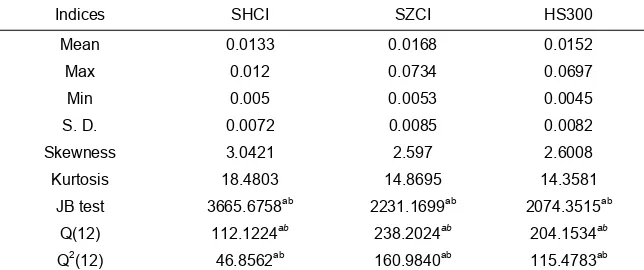
t low, are the daily highest and lowest price for day t , respectively.Table 1. Statistical characteristic of range series of three stock indices
Indices SHCI SZCI HS300
Mean 0.0133 0.0168 0.0152
Max 0.012 0.0734 0.0697
Min 0.005 0.0053 0.0045
S. D. 0.0072 0.0085 0.0082
Skewness 3.0421 2.597 2.6008
Kurtosis 18.4803 14.8695 14.3581
JB test 3665.6758ab 2231.1699ab 2074.3515ab Q(12) 112.1224ab 238.2024ab 204.1534ab
Q2(12) 46.8562ab 160.9840ab 115.4783ab
Notes: 1. S.D is abbreviated from standard deviation. 2. J-B test stands for the Jarque-Bera normality test for the distribution of the range series; 3. Q(12) and Q2(12) stand for the Ljung-Box Q test for up to 12th order serial correlation of the range series and squared range series. 4. a and b stand for rejection of the hypothesis at the 1% and 5% level, respectively.
3.2. Empirical Process and Results
The original range data are normalized into [0, 1] to improve the training efficiency of SVM. The normalized range data are classified into two subsections: the first 249 samples were taken for training the three models (SVM-SIWPSO, SVM-TVACPSO, SVM-TOOPSO model) and the remaining 69 samples are used for checking the out-of-sample forecasting performance. In order to describe the persistence of the range volatility, the range is calculated by the five most recent ranges.
4
In SVM-SIWPSO model, the parameters of SIWPSO algorithm are set as: m10,
max 0.9
, min0.1, c1c2 2, 0.02, and kmax20. In SVM-TVACPSO model, the
parameters of TVACPSO algorithm are set as: m10, wmax 0.9, wmin0.1, c1,ini2.5, c1,fin0.5
, c2,ini0.5, c2,fin2.5 and kmax20. In SVM-TOOPSO model, the parameters of TOOPSO
algorithm are set as: m10, wmax 0.9,wmin0.1, c10.2, c2 1.8and kmax 20. In order to
reduce the influence of stochasticity of three IPSO algorithms on parameters optimization, the parameters of SVM are optimized continuously by the three IPSO algorithms ten times, respectively. The optimal parameters obtained are adopted to construct SVM forecasting models. And then, the SVM models are employed to forecast range volatility one-step-ahead, respectively.
2where rˆt is the forecasted range volatility in checking samples, Rt is the corresponding
daily actual range. And N is the number of the checking samples. In addition, the time (TIME) for optimizing the parameters of SVM is recorded to evaluate the searching ability of the three IPSO algorithms.
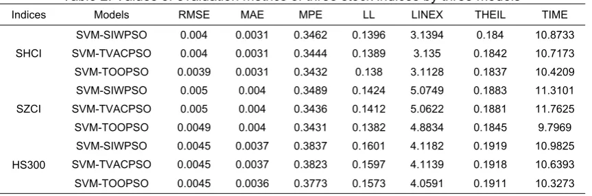
The evaluation results are given in Table 2. For SHCI and SZCI, SVM-TOOPSO model gives smaller RMSE, MPE, LL, LINEX, and THEIL but equal MAE relative to SVM-SIWPSO and SVM-TVACPSO models. For HS300, SVM-TOOPSO model gives smaller MAE, MPE, LL, LINEX, and THEIL but equal RMSE relative to the other two models. That indicates that SVM-TOOPSO model, as a whole, has better accuracy in range volatility forecasting than the other two models. For the three stock indices, SVM-TVACPSO model generates the smaller MPE, LL, LINEX, and THEIL than SVM-SIWPSO model except for RMSE and MAE, where it generates equal RMSE and MAE. That is to say, SVM-TVACPSO model obtains better accuracy in range volatility forecasting than SVM-SIWPSO model.
Table 2. Values of evaluation metrics of three stock indices by three models
Indices Models RMSE MAE MPE LL LINEX THEIL TIME
SHCI
SVM-SIWPSO 0.004 0.0031 0.3462 0.1396 3.1394 0.184 10.8733
SVM-TVACPSO 0.004 0.0031 0.3444 0.1389 3.135 0.1842 10.7173
SVM-TOOPSO 0.0039 0.0031 0.3432 0.138 3.1128 0.1837 10.4209
SZCI
SVM-SIWPSO 0.005 0.004 0.3489 0.1424 5.0749 0.1883 11.3101
SVM-TVACPSO 0.005 0.004 0.3436 0.1412 5.0622 0.1881 11.7625
SVM-TOOPSO 0.0049 0.004 0.3431 0.1382 4.8834 0.1845 9.7969
HS300
SVM-SIWPSO 0.0045 0.0037 0.3837 0.1601 4.1182 0.1919 10.9825
SVM-TVACPSO 0.0045 0.0037 0.3823 0.1597 4.1139 0.1918 10.6393
SVM-TOOPSO 0.0045 0.0036 0.3773 0.1573 4.0591 0.1911 10.3273
It is shown from TIME index that the time for finding the optimal parameters of SVM by TOOPSO algorithm is shorter than those of SIWPSO and TVACPSO algorithms for the three stock indices, which shows a better ability for optimizing the parameters of SVM in TOOPSO algorithm. Additionally, for SHCI and HS300, TVACPSO algorithm has shorter time for searching the optimal parameters of SVM compared to SIWPSO algorithm. For SZCI, the longer searching time are found in TVACPSO algorithm. In other words, on the whole, the searching ability of TVACPSO algorithm is superior to SIWPSO algorithm.
In summary, SVM-TOOPSO model provides best performance in rang volatility forecasting among the three models. In addition, SVM-TVACPSO model performs better than SVM-SIWPSO model.
Figure 1. Comparison of SHCI volatility forecasts with actual range volatility
Figure 2. Comparison of SZCI volatility forecasts with actual range volatility
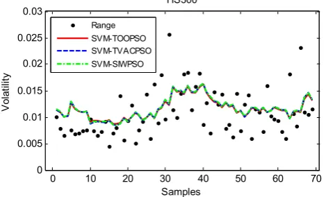
Figure 3. Comparison of HS300 volatility forecasts with actual range volatility
4. Conclusions
This paper combined SVM with three IPSO algorithms (SIWPSO, TVACPSO and TOOPSO) for forecasting range volatility. SVM was adopted to forecast the range volatility and the three IPSO algorithms were used to optimize the two parameters in SVM. The three stock indices of China stock market were analyzed to compare the forecasting ability of the proposed models. Empirical results indicate that SVM-TOOPSO model provides higher range volatility forecasting accuracy compared to SVM-SIWPSO and SVM-TVACPSO models. The ability of
0 10 20 30 40 50 60 70
0 0.005 0.01 0.015 0.02 0.025 0.03
Samples
V
o
la
tilit
y
SHCI
Range SVM-TOOPSO SVM-TVACPSO SVM-SIWPSO
10 20 30 40 50 60 70
0 0.01 0.02 0.03 0.04
Samples
V
o
la
ti
lit
y
SZCI
Range SVM-TOOPSO SVM-TVACPSO SVM-SIWPSO
0 10 20 30 40 50 60 70
0 0.005 0.01 0.015 0.02 0.025 0.03
Samples
Vo
la
ti
lity
HS300
TOOPSO algorithm is better than those of SIWPSO and TVACPSO algorithms in looking for the optimal parameters of SVM. Additionally, it is shown that SVM-SIWPSO model has higher accuracy and better searching ability in range volatility forecasting relative to SVM-SIWPSO model.
Acknowledgements
This work is supported by the Project Funded by China Postdoctoral Science Foundation (No. 2015M571194) and the Scientific Research Foundation of the Ministry of Education of China for Young Scholars (No. 11YJC790048).
References
[1] Bollerslev T. Generalized autoregressive conditional heteroscedasticity. Journal of Econometrics. 1986; 31(3): 307-327.
[2] Engle RF. Autoregressive conditional heteroskedasticity with estimates of the variance of United Kingdom inflation. Econometrica. 1982; 50(2): 987-1007.
[3] Donaldson RG, Kamstra M. An artificial neural network-GARCH model for international stock return volatility. Journal of Empirical Finance. 1997; 4(1): 17-46.
[4] Dadkhah M, Sutikno T. Phishing or hijacking? Forgers hijacked DU journal by copying content of another authenticate journal. Indonesian Journal of Electrical Engineering and Informatics (IJEEI). 2015; 3(3): 119-120.
[5] Tae HR. Forecasting the volatility of stock price index. Expert Systems with Applications. 2007; 33(4): 916-922.
[6] Bildirici M, Ersin ÖÖ. Improving forecasts of GARCH family models with the artificial neural networks an application to the daily returns in Istanbul Stock Exchange. Expert Systems with Applications. 2009; 36(4): 7355-7362.
[7] Hajizadeh E, Seifi A, Zarandi MHF, Turksen IB. A hybrid modeling approach for forecasting the volatility of S&P 500 index return. Expert Systems with Applications. 2012; 39(1): 431-436.
[8] Kristjanpoller W, Fadi A, Minutolo MC. Volatility forecast using hybrid neural network models. Expert Systems with Applications. 2014; 41(5): 2437-2442.
[9] Vapnik VN. An overview of statistical learning theory. IEEE Transactions on Neural Networks. 1999; 10(5): 988-999.
[10] Perez-Cruz F, Afonso-Rodriguez JA, Giner J. Estimating GARCH models using support vector machines. Quantitative Finance. 2003; 3(3): 1-10.
[11] Chen SY, Härdle WK, Jeong K. Forecasting volatility with support vector machine-based GARCH model. Journal of Forecasting. 2010; 29(4): 406-433.
[12] Gavrishchaka VV, Supriya B. Support vector machine as an efficient framework for stock market volatility forecasting. Computational Management Science. 2006; 3(2): 147-160.
[13] Wang BH, Huang HJ, Wang XL. A support vector machine based MSM model for financial short-term volatility forecasting. Neural Computing and Applications. 2013; 22(1): 21-28.
[14] Parkinson M. The extreme value method for estimating the variance of the rate of return. Journal of Business. 1980; 53(1): 61-65.
[15] Nair M P, Nithiyananthan K. Effective Cable Sizing model for Building Electrical Services. Bulletin of Electrical Engineering and Informatics. 2016; 5(1): 1-8.
[16] Hu JX, Zeng JC. A particle swarm optimization model with stochastic inertia weight. Computer Simulation. 2006; 23(8): 164-167.
[17] T Sutikno, M Facta, GRA Markadeh. Progress in Artificial Intelligence Techniques: from Brain to Emotion. TELKOMNIKA (Telecommunication Computing Electronics and Control). 2011; 9(2): 201-202.
[18] Chaturvedi KT, Pandit M, Srivastava L. Particle swarm optimization with time varying acceleration coefficients for non-convex economic power dispatch. Electrical Power and Energy Systems. 2009; 31(6): 249-257.
[19] Bhargavi VR, Senapati RK. Bright Lesion Detection in Color Fundus Images Based on Texture Features. Bulletin of Electrical Engineering and Informatics. 2016; 5(1): 92-100.