Full Length Research Paper
Identification and non-linear control strategy for
industrial pneumatic actuator
M. F. Rahmat
1, Sy Najib Sy Salim
2, N. H. Sunar
1,
Ahmad
‘
Athif Mohd Faudzi
3, Zool Hilmi
Ismail
3and K. Huda
41
Department of Control and Instrumentation Engineering, Faculty of Electrical Engineering, Universiti Teknologi Malaysia, 81310 Skudai, Malaysia.
2
Department of Control, Instrumentation and Automation, Faculty of Electrical Engineering, Universiti Teknikal Malaysia Melaka, Hang Tuah Jaya, 76100 Durian Tunggal, Melaka Malaysia.
3
Department of Mechatronics and Robotics Engineering, Faculty of Electrical Engineering, Universiti Teknologi Malaysia, 81310 Skudai, Malaysia.
4
Department of Automotive, Faculty of Mechanical Engineering, Universiti Teknikal Malaysia Melaka, Hang Tuah Jaya, 76100 Durian Tunggal, Melaka Malaysia.
Accepted 17 February, 2012
In this paper, a combination of nonlinear gain and proportional integral derivative (NPID) controller was proposed to the trajectory tracking of a pneumatic positioning system. The nonlinear gain was employed to this technique in order to avoid overshoot when a relatively large gain is used to produce a fast response. This nonlinear gain can vary automatically either by increasing or decreasing depending on the error generated at each instant. Mathematical model of a pneumatic actuator plant was obtained by using system identification based on input and output of open-loop experimental data. An auto-regressive moving average with exogenous (ARMAX) model was used as a model structure of the system. The results of simulation and experimental tests conducted for pneumatic system with different kind of input namely step, sinusoidal, trapezoidal and random waveforms were applied to evaluate the performance of the proposed technique. The results reveal that the proposed controller is better than conventional PID controller in terms of robust performance as well as show an improvement in its accuracy.
Key words: Pneumatic positioning systems, nonlinear PID, identification, real time implementation.
INTRODUCTION
Currently, pneumatic actuator drives have been widely used in various industrial applications including those involve in the manufacturing and processing of automation. This is due to several factors such as easy maintenance, low cost, clean operating environment, durability, robustness, high power-to-weight ratio and free from overheating in the case of constant load (Hildebrandt et al., 2010; Kaitwanidvilai et al., 2011; Noor et al., 2011; Rahmat et al., 2011a). Pneumatic actuator is also an alternative to the hydraulic actuator and servo motor,especiallyinhandlingtaskswhereitcaneffectively reduce the costs (Messina et al., 2005). It is also suitably
*Corresponding author. E-mail: [email protected].
used as a tool to study human convenience, such as, to facilitate investigation of chair shapes (Faudzi et al., 2010). In spite of these advantages, pneumatic actuators are subject to nonlinearities in which the precise position control of this actuator is difficult to achieved due to compressibility of air, valve fluid flow characteristics and the highly nonlinear behaviour of friction effects at near-zero velocities (Khayati et al., 2009). The first theoretical basis of the pneumatic system dynamic control was initially made by Shearer (1956) which the dynamic of the system is derived through nonlinear differential equation and then followed by linear mathematical model.
2566 Int. J. Phys. Sci.
2011; Kaitwanidvilai et al., 2011; Khayati et al., 2009; Kothapalli and Hassan, 2008; Ning and Bone, 2005; Richer and Hurmuzlu, 2001b; Wang et al., 1999), among others. Most of them dealt with the control of double acting cylinder. As stated previously, the dynamic model of the pneumatic actuator is characterized by significant nonlinearities. Therefore, the use of standard linear controller is usually not able to give good performance for the system. On this grounds, alternative control strategies based on fuzzy control laws (Jakub et al., 2009; Kaitwanidvilai et al., 2011), sliding mode control methodology (Bone and Ning, 2007; Paul et al., 1994; Richer and Hurmuzlu, 2001b; Tsai and Huang, 2008b), neural network (Hassan, 2010) and back stepping design methodology (Rao and Bone, 2008) have been success-fully tested. Since this paper involves control strategy, some relevant papers that emphasized controller design has been studied and described briefly here.
Hamiti et al. (1996) has taken an approach to alter third-order system for a pneumatic actuator into three first-order systems that are connected in series. In their research, the original integrator plant transfer function of the system was modified by inserting an analogue feedback with proportional gain k. The proportional gain k is tuned until the greatest value of gain k which leads the system to the verge of the appearance of overshoot is obtained. In this circumstance, the system is said to be critically damped so that the response of this third-order model can be approximated by a first-order system with some amount of dead time. Furthermore, the system was controlled using proportional-integral (PI) controller in which the Chien-Hrones-Reswick tuning formulas were applied in order to determine the parameters of the controller. In addition, the weighted function was added to the integral gain to prevent the system from stick and slip near the reference which is occurred due to the presence of stiction.
In another research, van Varseveld and Bone (1997) made modifications to the proportional integral derivative (PID) compensation by adding the friction compensation, bounded integral action and position feed forward. The impact of this consolidation has shown that the controller is robust to a six fold increase in the system mass and able to follow the S curve trajectory smoothly without effect the steady state accuracy. Moreover, the results indicate that the use of friction compensation was victorious to reduce the steady state error to almost 40%. In a subsequent study, Bone and Ning (2007) managed to increase the performance of the pneumatic system through a sliding mode control method based on linearized plant and nonlinear plant model which is simply called SMCL and SMCN, respectively. The controller was tested to the system for both horizontal and vertical movement. The results for the root-mean-square error (RSME) and tracking error indicate that the performance of SMCN is better than SMCL for both cases. Regarding the durability tests, the SMCL was found more robust in
the case of the actual payload and greater than nominal payload. Meanwhile, in the case of the actual payload is smaller than the nominal payload, SMCN was proven to be more robust.
As noted, one of the difficulties in the control of pneumatic servo systems is the presence of uncertainties in the parameters of the system. Due to this reason, Tsai and Huang (2008b) proposed a multiple-surface sliding controller (MSSC) in which one of the objectives is to take care of the mismatched uncertainties. Based on the reported results, the proposed strategy was able to provide good performance regardless of the time-varying payload and other uncertainties. In another paper, a function approximation technique (FAT)-based adaptive controller was previously proposed by the same researchers for pneumatic servo systems with variable payload and uncertain disturbances (Tsai and Huang 2008a). The researchers claimed that the satisfactory tracking performances were achieved for the slow motion tracking. Conversely, a slightly larger deviation occurred for the fast motion. The closed loop stability for both strategies was proved with the Lyapunov method.
One of the factors that contribute to the nonlinearities of the pneumatic system is a friction force acting on the piston. Due to this consideration, Schindele and Aschemann (2009) conducted an experiment by adding LuGre observer. Here, an adaptive back stepping con-troller was implemented in order to update and estimate the unknown parameters of the observer. Referring to the experimental results, the performance of the system indicates an improvement in terms of point to point steady-state error. However, the tracking performance of the system reveals that this controller is not so robust referring to the augmented error that occurs even on a slight increase in load.
Based on the previous literature, most of the studies that have been conducted within the last 10 years were focused on the use of quite complicated controllers for the purpose of overcoming problems caused by the uncertainty of the parameters as well as by the frictional force. Most of these control technique involves many parameters which is engage with complicated mathematical equation. Owing to this reason, most the industries still employ the control loops based on proportional-integral-derivative (PID) controller because of its simplicity, robustness and easy to understand even though it might be difficult to deal with highly nonlinear system.
Displacement
transducer
2468101214161820
0 20 40 60 80 100
y
Cylinder
Slide Table Chamber A
Chamber B
Magnetic
Sensor
Proportional valvePs
DAQP
AP
Bu
Pressure
sensor
Pressure
sensor
P
0P
0L=500 mm
Payload
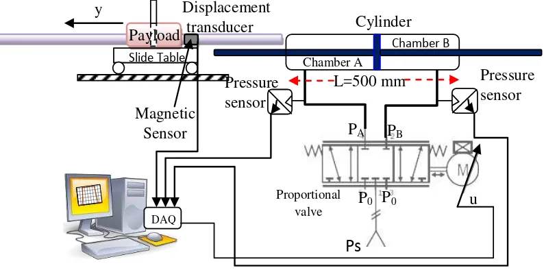
Figure 1. Pneumatic positioning system.
prevent an oscillation and overshoot. The simulations and experiments is performs to confirm the capability of this controller. The simulation and experimental results prove that the automatic nonlinear gain is able to make the PID controller more robust to the load changes for both position and tracking performance.
The paper is organized as follows. A modelling of the pneumatic actuator system based on fundamental physical derivation and followed by model identification is described in next section. It then continued by a description of the controller design and the development of a NPID controller. The experimental setup for the pneumatic actuator system is provided in the following section. Meanwhile the results for both simulation and experimental is shown in the following discussion. Sub-sequently, the performances of the proposed controller based on positioning and tracking are described. Concluding remarks of the research are stated in the last section.
PLANT MODEL
Mathematical modelling description of pneumatic system
In this research, a pneumatic system that composed of double-acting actuator, 5/3 proportional directional control valve and mass payload as shown in Figure 1 was considered. The description of how the mathematical model of a pneumatic servo system can be derived is clearly described here. The nonlinear dynamics of a pneumatic servo system can be derived through combination of fluid dynamics, thermodynamics and the dynamics of motion. The condition of air in the cylinder
chamber is determined by pressures (PA and PB),
volumes of chambers (VA and VB) and corresponding
temperatures of air (TA and TB). The mass flow rate of a
compressible fluids is refers as a function of the ratio between downstream and upstream pressure taken at the control valve orifice. The dynamics of motion is described base on Newton Laws. Here, several assumpt-ion have been taken into consideratassumpt-ion (Bigras and Khayati, 2002) which are;
1. Gas is ideal,
2. Gas density is uniform in the chamber and in the pipe, 3. Gas in the chamber and in the pipe are isothermal, 4. Flow in the servo valve and in the connection port are isentropic with negligible temperature variation,
5. Flow leakages are negligible in the servo valve.
Based on isentropic flow assumptions, the compressible
mass flow rate,
m
through a valve orifice can be described as (Rahmat et al., 2011a; Richer and Hurmuzlu, 2001a): ) ( 1 2 . . . ) ( 1 . . . 1 2 . . ) , ( 1 1 1 1 2 1 sonic P P P if k R k T P A C subsonic P P P if P P P P T P k R k A C P P m cr u d k k u v f cr u d k k u d k u d u v f d u (1) 1
1
2
k k crk
P
(2)where PuandPd are upstream and downstream pressures,
respectively, m P P
u, d
is the mass flow rate,f
2568 Int. J. Phys. Sci.
nondimensional discharge, Avis the effective area of the
valve orifice,
T
is the temperature, R is the gas constant,k
is the specific heat ratio and Pcr is the critical pressurewhich can be determined based on Equation 2. Due to the assumption that, there is no change in the total heat energy of the gas under compression, the specific heat ratio for air is k=1.4. According to Beater (2007), by referring to the standard ISO 6358, with a relative humidity of 65%, the value of gas constant (R), temperature (T) and ambient pressure (Po) are 288
J/(kg.K), 293.15 K and 100 kPa, respectively. The effective area of the valve orifice (AV) has been
expressed in various approaches by the previous researchers. Here, the approach describes by Kothapalli and Hassan (2008) was considered in which the relationship between the effective area and the control spool movement can be expressed as:
4
2spool V
X
A
(3)
The relationship between spool movement and the voltage input is:
u
C
X
spool
v (4)Where, Xspoolis the spool displacement, CV is the valve
constant and u is the voltage input.
The upstream and downstream pressures are different from the charging and discharging process of the cylinder chamber according to the following functions:
)
,
(
,A S A
i
m
P
P
m
(5))
,
(
,A A a
o
m
P
P
m
(6))
,
(
,B S B
i
m
P
P
m
(7))
,
(
,B B a
o
m
P
P
m
(8)Where, mi A,
and mi B,
are the mass flow rates into cylinder
chamber A and B respectively, whereas mo A,
and mo B,
are the mass flow rate leave from cylinder chamber A and B respectively, PAand PB are the pressure inside chamber
A and B respectively, PSis the supply pressure and Pais
the ambient pressure. Equation 5 and 7 represent the charging process where the pressure in the supply tank and the cylinder chamber are considered to be upstream
and downstream, respectively. Whereas, for discharging process as represented in Equation 6 and 8, the pressure in the chamber is the upstream and the ambient pressure is the downstream pressure. The status of the flow can be classified as either choked flow or under-chocked flow depending on the downstream pressure Pd and the
upstream pressure (Pu)of the orifice. Choked flow occurs
in pneumatic system when Pd/Pu is less than the critical
pressure ratio Pcr.
With the assumption of air as a perfect gas undergoing an isothermal process, the dynamics of the pressures in two chambers of the pneumatic cylinder can be represented as shown in Equation 9:
( , ) ) , ( ) , ( ) , ( ) , ( ) , (.
.
B A B A B A B A o B A i B AV
V
P
k
m
m
V
k
T
R
P
(9)
Where, P(A,B) is the pressure inside chamber A and B,
) , (AB
P
is the rate of change in pressure inside chamber
A and B,
i
m
is the inlet mass flow rate to both chambers,o
m
is the outlet mass flow rate from each chamber, V is
the volume of each chamber and
V
(A,B)
is the rate of change in volume for each chamber. The volume of chamber A and B can be expressed as:
)
.(
x
A
V
A
(10))
.(
L
x
A
V
B
(11)Where, x is the piston position, L is the piston stroke and A is the piston area.
The equation of motion for piston rod including the mass and friction effects of pneumatic cylinder can be
expressed using Newton’s second law as:
r a B B A A L f P
L
M
x
F
F
P
A
P
A
P
A
M
)
(
(12)
Where, ML and MP is the external load mass and piston
rod mass, respectively, Ff is the friction force, FL is the
external force, Ar is the rod cross sectional area and Pa
represent the atmospheric pressure. The LuGre friction model proposed by Canudas et al. (1995) is one of the prominent model that has always been used in research (Rahmat et al., 2011b; Richer et al., 2001a). The friction force (Ff), dynamics of the internal state (z) and stribeck
1
(
)
C z
1
(
)
B z
1
1(
)
A z
+
e(k)
u(k)
y(k)
Figure 2. ARMAX model stracture.
Bv
z
z
F
f
1
0
(13)z
v
g
v
v
z
)
(
0
(14) 0 2).
(
)
(
vs v C SC
F
F
e
F
v
g
(15)v
B
v
e
F
F
v
F
v
B
v
v
g
F
s v v C S C f.
)
sgn(
).
(
)
sgn(
.
)
sgn(
)
(
2 0
(16)Where, z is the friction internal state,
0is the stiffnesscoefficient,
1is the damping coefficient, B is the viscous friction, Fc is the Coulomb friction and Fs is the staticfriction.
Model identification
Identification of dynamic systems is the process of obtaining mathematical model through experiments on the plants that viewed as a black box based on excitation and response signals. Through this process, a number of parameters may be generated and subsequently the model of the system can be determined. In this study, experiments were conducted starting with collecting the input and output data based on open loop system with sampling frequency of 100 Hz. The input signal with multi amplitude and frequency sine wave as shown in Equation 17 is used where 2000 numbers of data have been
collected. The collected data is split into two parts which is model estimation and model validation. The first procedure is to estimate the model and then followed by validation. This model is vital due to model experimental verification later. An ARMAX model which is describe by Equation 18 is used as a model structure of the system. Through this model structure, the deterministic and stochastic parts of the system can be modelled. Figure 2 illustrates the structure of ARMAX model.
t
tt
Vin0.5cos(2(0.05))1.5cos0.2 )2.5cos2 (17)
z y
k B
z u
k C
z e
kA 1 1 1 (18)
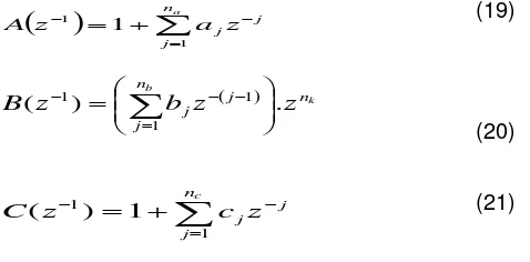
Where, u(k), y(k) and e(k) represent the sampled excitation, noise corrupted response signal and white noise sequence respectively. While, A, B and C are
monic polynomials in the time-shift operator
z
1 and can be defined as Equation 19, 20 and 21, respectively:
na
j j jz a z A 1 1 1 (19)
k
b
n n
j
j
jz z
b z
B( ) .
1 1 1
(20)
nc
j j jz c z C 1 1 1 )
( (21)
Where,
n
ais the number of poles,n
bis the number ofzeroes plus,
n
cis the number of C polynomial coefficient2570 Int. J. Phys. Sci.
Am
p
li
tu
d
e
(m
m
)
Time (s)50 55 60 65 70 75 80 85 90 95 100
-200 -150 -100 -50 0 50 100 150 200
Measured and simulated model output
Am
p
li
tu
d
e
(V
o
lt
)
Time (s)50 60 70 80 90 100
-4 -2 0 2
4 1 V = 50mm
(a)
(b)
Figure 3. Input and output signal; (a) multi-sine input, (b) best fit graph of the estimated model (output).
-20 -15 -10 -5 0 5 10 15 20
-0.3 -0.2 -0.1 0 0.1 0.2
Autocorrelation of residuals for output y1
-20 -15 -10 -5 0 5 10 15 20
-0.2 -0.1 0 0.1 0.2 Samples
(a)
(b)
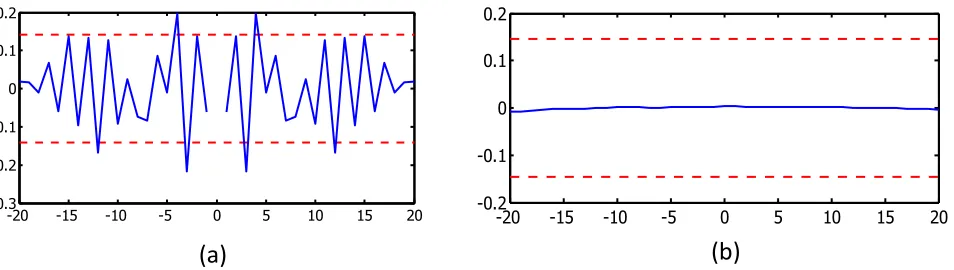
Figure 4. Residual analysis; (a) autocorrelation of residuals, (b) cross correlation.
this selection, the monic polynomials in the time-shift
operator
z
1 that acquired from system identification are defined as follows:
1 1 2 39177
.
0
827
.
2
909
.
2
1
z
z
z
z
A
3 2 1 15834
.
0
183
.
1
6045
.
0
)
(
z
z
z
z
B
1 1 2 34925
.
0
049
.
1
554
.
1
1
z
z
z
z
C
Referring to Equation 18, it can be seen clearly that the ARMAX model consists of two transfer functions which is between input and output as well as between noise and output. Based on these monic polynomials, the discrete transfer function of the system can be obtained. In addition, the continuous transfer function can be obtained using zero order hold (ZOH) conversion method with sampling time, Ts= 0.01s. This conversion method generates the continuous time input signal by holding
each sample value constant over one sample period. Based on the result from system identification, the transfer function for dynamics of the system in discrete G(z) and continuous G(s) form which can be represented as follows:
9177
.
0
827
.
2
909
.
2
5834
.
0
183
.
1
6045
.
0
2 3 2
z
z
z
z
z
z
A
z
B
z
G
1003
.
0
25
.
90
585
.
8
4851
6
.
220
98
.
61
2 3 2
s
s
s
s
s
s
G
Figure 5. Block diagram of the N-PID control system.
within the tolerance band ±0.1. Besides, ARX and NARX model are also tested as a comparison in this research. The validation data show that the best fit of ARX model was 84.07% with loss function 0.0484522, while for NARX model, the best fit and loss function were 90.29% and 0.043747, respectively. Based on these results, it can be concluded that the ARMAX model is better compared to ARX and NARX model. The modelling simulation was carried out using Matlab-Simulink package.
CONTROLLER DESIGN
The classical PID controller emphasizes a straight forward design procedure in order to achieve the favourable result in controlling the position and continuing motion as the ultimate goal. However, as the position control performs more rigorously, this type of controller is often difficult to gives the good performance due to the presence of nonlinearities especially in pneumatic systems. In order to overcome this problem, many control strategies have been investigated by researchers such as sliding mode control, fuzzy logic control, adaptive control, robust control and others. However, most of these control strategies are not implemented in industries as they prefer to use PID controller due to its simplicity, low cost and easy to operate. In this paper, the PID controller that incorporates with automatic nonlinear gain was designed, simulated and tested to control the position and tracking of pneumatic actuator. The automatic nonlinear gain is used to accommodate the nonlinearity as well as to overcome the deficiencies in classical PID controller. This control technique is viewed as one of the simple strategy for industrial application and it is quite effective to reach the performance which is unable to be achieved by a
linear classical PID controller.
The automatic gain adjustment used in this study could produce a rapid response without producing a significant overshoot. The gain is automatic changeable depend on the error between the commanded and actual values of the controlled variable. In this case, when the error is large, the gain will increase significantly to make a large corrective action and subsequently, while the error diminishes, the gain will reduced automatically. This can drive the system output to its goal rapidly without significant overshoots as well as able to prevent excessive oscillations (Su et al., 2005). Besides, the non-linear PID controller can be use as friction compensation and it also talented to generate the better tracking performance (Armstrong et al., 2001).
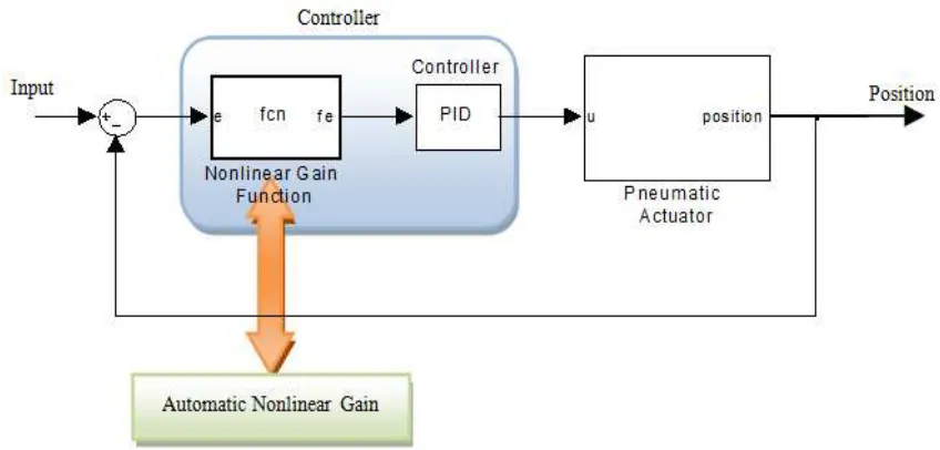
Nonlinear PID (N-PID) controller
The proposed nonlinear PID (N-PID) controller consists of a sector bounded nonlinear gain, k(e) which is combine in cascade with PID controller, as shown in Figure 5. The parameters of the linear PID controller are obtained based on previous work (Rahmat et al., 2011a). The automatic gain adjustment k(e) act as a nonlinear function of error e(t), that is bounded in the sector
max
0k e k e as indicated in Equations 22 and 23.
These are identified as the range of options available for the nonlinear gain, k(e). The output produced from this nonlinear function is known as a scaled error and can be expressed as Equation 24. Subsequently, the whole equation of the N- PID controller can be written as revealed in Equation 25.
2 exp
exp e e
e
2572 Int. J. Phys. Sci.
-0.06
-0.04
-0.02
0
0.02
0.04
0.06
-0.8
-0.6
-0.4
-0.2
0
0.2
Real (Re)
Im
a
g
in
a
ry
(
Im
)
0.035
Figure 6. Popov plot of the N-PID control system.
Figure 7. Relationship between various nonlinear gain and error.
max max
max
e
e
e
sign
e
e
e
e
e
j G e
k max 1
(23)
e
k
e
e
t
f
.
(24)0
( ) PID p[ ( ) ( )] p t[ ( ) ( )] p d [ ( ) ( )] I
k d
f e u k k e e t k e e t dt k T k e e t
T dt
(25)
From Equation 22,α is represents the rate of variation of nonlinear gain, while emax is a range of variation. In this
study, the value of α and emax are decided to be 11 and
0.14, respectively. The selection of parameters α and emax depend on the maximum value of nonlinear gain k(e)
which is determined based on the range of the gain for stability.
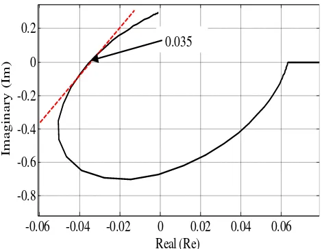
The Popov stability criterion is used in determining the maximum value of k(e). The procedures to determine the range of k(e) by using Popov stability criterion has been discussed in detail in previous research (Seraji, 1998). By using Matlab software, the Popov plot of G(j) is crossing the real axis at the point (-0.035, j0) as shown in Figure 6. Based on this information, the maximum value of the nonlinear gain k(emax) can be obtained through Equation
23. Therefore, according to the Popov stability criterion, the range of the allowable nonlinear gain k(e) is (0, 28.57).
Besides stability, the presence of chattering is also needed to be taken into account when determining the value of k(emax). This can be solved by refining the value
of k(emax) manually according to the range of allowable
until an appropriate value is obtained. In this case, the appropriate value of k(emax) are 2.44. Subsequently,
based on this value the parameters of α and emax can
determined according to Equation 22. Here, the value of emax was be selected first and then based on this value
the parameter of α can be calculated. In order to avoid an overshoot, emax should be selected in a small value.
Figure 7 demonstrate the variation of k(e) with respect to the error changes due to these selected value of the parameters of α and emax. It can be seen that the value of
nonlinear gain k(e) is equal to 1 when the error, e=0. In this situation, the controller seems to function as a conventional PID controller. In other words, the nonlinear gain k(e) is only participating when there is the presence of errors.
EXPERIMENTAL SETUP
A schematic view of the pneumatic system under consideration is shown in Figure 1. The hardware designed is quite flexible in which the payload mass, type of cylinder and the orientation of movement can be changed easily.
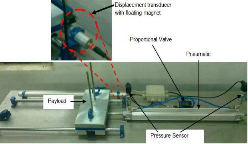
Figure 8 show the photograph of the experimental setup used to validate the proposed method. The system under consideration consists of:
1. 5/3 bi-directional proportional control valve (Enfield LS-V15s) with bandwidth 100Hz;
2. Double rod cylinder with stroke and diameter 0.5 m and 40 mm, respectively;
3. Non contact micropulse displacement transducer with floating Magnet (Balluff BTL6) and analog output signal in the range of 0 to 10 v;
4. Data acquisition card (NI-PCI-6221 card), 5. Pressure sensors (WIKA S-11)
6. PC with Matlab as a platform to implement the controller and 7. Air compressor supply.
Figure 8. Pneumatic system mechanism tested setup.
Table 1. Controller gains including rate variation of nonlinear gain and range of variation.
Parameter Value
Proportional gain (kp) 5.74
Integral gain (ki) 0.25
Derivative gain (kd) 0.13
Rate variation of nonlinear gain (α) 11 Range of variation, (emax) 0.14
RESULTS AND DISCUSSION
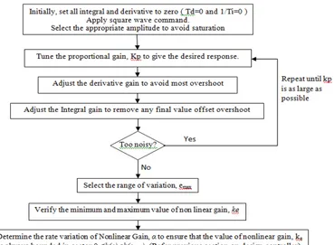
Here, a N-PID controller and conventional PID controller are employed to the actual pneumatic actuator system to evaluate the performance of both cases. The results from both simulation and experimental are clearly shown in this paper. The parameters of the controller including rate variation of nonlinear gain (α) and the range of variation of error (emax) are tabulated in Table 1. In order to design
the controller, the parameters of the PID controller were required to determine earliest before the rate variation of nonlinear gain (α) as well as the range of variation error (emax) can be determined. The procedures to obtain the
parameters are shown in Figure 9. The explanation on how to determine the parameters which depends on the lower bounded and upper bounded of the nonlinear gain (ke) is described in previously under sub-topic of
controller design. Figure 10 shows the implementation block diagram of the real system that was interfaced through data acquisition (DAQ) card. Both simulations
and experiments were performed with four types of input reference, namely: step, trapezoidal, sinusoidal and random functions as shown in Figures 11, 12, 13 and 15, respectively.
2574 Int. J. Phys. Sci.
Figure 9. Procedure to obtain the parameters of the controller.
Figure 10. Implementation block diagram of the real system.
Po
sitio
n
(m
m
)
Time (s)
5 10 15 20
0 50 100 150
Reference PID
NPID
Actual response
NPID Simulation response
6 8 10 12 14 16 18 0
20 40 60 80 100
15.8 15.9 16 16.1 16.2 16.3 45
50 55 60 65 70
Input
NPID
PID
Po
sitio
n
(
m
m
)
Time (s) 2 4 6 8 10 12 14 16 18 20
0 20 40 60 80 100
15 15.5 16 75
80 85 90 95 100
Simulation
Experiment
Time (s)
(a)
Time
(s)
(b)
Figure 12. Results based on trapezoidal input reference; (a) simulation results for NPID and PID (b) comparison between simulation and experimental result of NPID controller.
10 15 20 25 30 35
-100 -50 0 50 100
Reference
NPID PID
Time (s)
10 15 20 25 30
-100 -50 0 50 100
Reference
NPID PID
Po
sitio
n
(
m
m
)
Time (s)
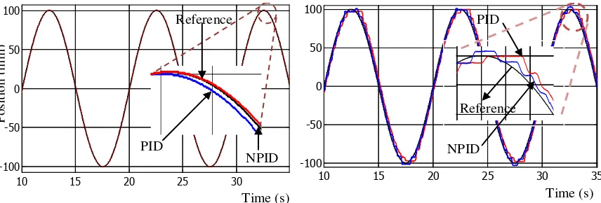
Figure 13. Results based on sinusoidal input reference; (a) simulation results for NPID and PID (b) comparison between simulation and experimental result for NPID and PID controller.
signal based on trapezoidal wave, confirming the effect of using automatic nonlinear gain on the conventional PID controller. Besides, for further verification of NPID controller performance, the sine wave with the various frequencies and amplitudes were realized. Figure 15 shows the results for this experiment, where the frequency was initially set to 0.2 Hz with strokes of -70 to 70 mm and -50 to 50 mm. Subsequently, starting at 40 s, the frequency was abruptly changed to 0.1 Hz with the initial stroke of 50 to 50 mm and followed by stroke of -100 to -100 mm. Based on the results obtained, the proposed controller was able to track the demand even though the frequency or amplitude or both changed all of the sudden.
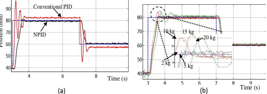
The mismatch between the nominal and actual payload mass was also tested in order to investigate the robust-ness of the proposed controller. To prove that the system is robust, some experiment were conducted, where various payload including 2, 5, 8, 10, 12, 15 and 20 kg were added on a carriage with about 0.5 kg mass that
2576 Int. J. Phys. Sci.
6 8 10 12 14 16
-0.4 -0.2 0 0.2 0.4 0.6
NPID Error
PID Error
Po
siti
on
e
rr
or
(m
m
)
Time (s)
Figure 14. Experimental result of position error signal based on trapezoidal reference signal.
Time (s)
10 20 30 40 50 60 70 80
-100 -50 0 50 100
0 50
0.2 Hz 0.1 Hz
0 0 0 20 40 60
Po
sitio
n
(m
m
)
Figure 15. Experimental results of various frequencies and amplitudes (based on sinusoidal reference) with abruptly change.
4 6 8
40 50 60 70 80 90
P
o
siti
o
n
(m
m
)
Time (s)
Conventional PID
NPID
(a)
(b)
3 4 5 6 7 8 9
40 50 60 70 80
78 80 82 84
Time (s)
15 kg 10 kg
2 kg 5 kg
20 kg
4 6 8 10 12 14 16 18 20 0
20 40 60 80 100
Time (s)
Po
s
itio
n
(
m
m
)
10 kg 8 kg
Time (s)
4 6 8 10 12 14 16 18
0 50 100 150
2 kg 5 kg
(a)
(b)
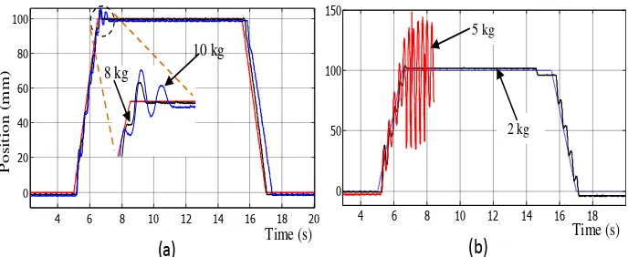
Figure 17. Experimental results of different payload based on trapezoidal input reference (a) NPID (b) conventional PID controller.
(a) (b)
10 20 30 40 50 60
-150 -100 -50 0 50 100 150
32.5 33 33.5 110
120 130 140 150 160
Time (s)
Po
sitio
n
(
m
m
)
50 55 60 65 70 75 80
-100 -50 0 50 100
8 kg
5 kg 8 kg 10 kg 15 kg 20 kg
Time (s)
0 0.5 1 1.5
-50 0 50 100 150
5 kg
Figure 18. Experimental results of payload up to 20 kg based on sinusoidal input reference; (a) NPID controller can well accommodate a payload up to 20 kg, (b) conventional PID controller cannot sustain when the payload increase more than 5 kg.
Figures 17b and 18b where the response of the system was getting worse and the experiment failed to continue.
The robust performance of the proposed controller is shown seen in Table 2. The results indicate that the proposed technique was capable to handle the load up to 20 kg for all three types of signal that was applied. The performance of the system due to the step input prove that the pneumatic actuator controlled by NPID produced a good result referring to a slight overshoot that occurs, although when the load is increased significantly. In addition, based on changes in the measurement of the integral absolute error (IAE), the distinction of per-formance between NPID and conventional PID controller can be clearly observed as shown in Figure 19. Based on this distinction, it can be supposed that the NPID controller has perform better compared to conventional PID controller.
CONCLUSION
In this paper, a nonlinear PID control technique was
proposed and applied to the trajectory of a pneumatic positioning system. Simulations and experiments were conducted to verify the performance of the proposed technique. It was demonstrated that the nonlinear gain which is combine in cascade with PID controller can make the system more robust and capable to minimise the positioning error as well as able to reduce the overshoot. The experimental results also confirmed that the performance of the system with NPID controller was significantly enhanced due to its capability to perform with load up to 20 kg compared to the conventional technique where it failed to perform for load greater than 5 kg. The performance indices as listed in the results prove that the proposed controller is capable to make the pneumatic servo system more robust against the load changes.
ACKNOWLEDGMENTS
2578 Int. J. Phys. Sci.
Table 2. Comparison of the performance for pneumatic actuator controlled by nonlinear PID (NPID) and conventional PID based on the load variation.
Load (kg)
Step Sinusoidal Trapezoidal
% OS NPID
Ess (mm) IAE % OS
PID
Ess (mm) IAE NPID IAE PID IAE NPID IAE PID IAE
0.5 0 0.5 35.12 8.03 2.2 37.31 37.91 60.27 30.48 36.75
2 0 0.5 39.53 16.46 2.4 42.24 38.79 61.66 25.60 39.04
5 0 0.5 40.84 System oscillate 232.60 48.26 245.6 27.82 255.2
8 3.75 0.5 41.91
System unstable
47.18
System unstable
33.49
System unstable
10 5.68 1 45.23 55.50 48.76
12 5.69 1 48.45 58.41 51.13
15 5.70 1 51.74 62.93 56.94
20 5.69 1 56.11 69.72 67.73
load (kg)
Controlled by NPID
Controlled by conventional P
Step
Trapezoidal
Sinusoidal
Perf
o
rm
an
ce
i
nd
ex,
IAE
Figure 19. The variation of performance index, IAE with respect to the load changes.
(UTeM) through Research University Grant (GUP) Tier 1 votenumberQ.J130000.7123.00H36.Authorsaregrateful to the Ministry, UTM and UTeM for supporting the work.
REFERENCES
Armstrong B, Neevel D, Kusik T (2001). New results in NPID control: Tracking, integral control, friction compensation and experimental results. IEEE Trans. Control Syst. Technol., 9(2): 399-406.
Beater P (2007). Pneumatic Drives (System Design, Modeling and Control). Verlag Berlin Heidelberg: Springer: pp. 6-10.
Bigras P, Khayati K (2002). Nonlinear observer for pneumatic system with non-negligible connection port restriction. Presented at Proceedings of the American Control. Conference, pp. 3191-3195. Bone GM, Ning S (2007). Experimental Comparison of Position
Tracking Control Algorithms for Pneumatic Cylinder Actuators. IEEE/ASME Transactions on Mechatronics, 12(5).
Canudas DWC, Olsson H, htrom KJ, Lischinsky P (1995). A New Model for Control of Systems with Friction. IEEE Transact. Automat. Control., 40(3): 419-425.
Faudzi AAM, Suzumori K, Wakimoto S (2010). Development of an Intelligent Chair Tool System Applying New Intelligent Pneumatic Actuators Advanced Robotics, 24(10): 1503-1528.
Hamiti K, Voda-Besancon A, Roux-Buisson H (1996). Position Control of a Pneumatic Actuator under the Influence of Stiction. Control Eng. Pract., 4(8): 1079-1088.
Hassan MY (2010). A Neural Network Based Fuzzy Controller For Pneumatic, Circuit. Eng. Tech. J., 28(4): 793-806.
Hildebrandt A, Neumann R, Sawodny O (2010). Optimal System Design of SISO-Servopneumatic Positioning Drives, IEEE Trans. Control. Syst. Technol., 18(1): 35-44.
Jakub E, Takosoglu RFD, Laski PA (2009). Rapid prototyping of fuzzy controller pneumatic servo-system. Int. J. Adv. Manuf. Technol., 40: 349-361.
of freedom (DOF) pneumatic robot. Int. J. Phys. Sci., 6(23): 5575-5585.
Kaitwanidvilai S, Olranthichachat P (2011). Robust loop shaping-fuzzy gain scheduling control of a servo-pneumatic system using particle swarm optimization approach. Mechatronics, (21): 11-21.
Khayati K, Bigras P, Dessaint L-A (2009). LuGre model-based friction compensation and positioning control for a pneumatic actuator using multi-objective output-feedback control via LMI optimization. Mechatronics, 19(4): 535-547.
Kothapalli G, Hassan MY (2008). Design of a Neural Network Based Intelligent PI Controller for a Pneumatic System. IAENG Int. J. Comput. Sci., 35(2).
Messina A, Giannoccaro NI, Gentile A (2005). Experimenting and modelling the dynamics of pneumatic actuators controlled by the pulse width modulation (PWM) tech. Mechatr., 15(7): 859-881. Ning S, Bone GM (2005). Development of a nonlinear dynamic model
for a servo pneumatic positioning system. Presented at IEEE International Conference on Mechatronics and Automation, pp. 43-48.
Noor SBM, Ali HI, Marhaban MH (2011). Design of combined robust controller for a pneumatic servo actuator system with uncertainty. Sci. Res. Essays, 6(4): 949-965.
Paul AK, Mishra JE, Radke MG (1994). Reduced order sliding mode control for pneumatic actuator. IEEE Trans. on Control. Syst. Technol., 2(3): 271-276.
Rahmat MF, Salim SNS, Faudzi AAM, Ismail ZH, Samsudin SI, Sunar NH,Jusoff K (2011a). Non-linear Modeling and Cascade Control of an Industrial Pneumatic Actuator System. Aust. J. Basic Appl. Sci., 5(8): 465-477.
Rahmat MF, Zulfatman, Husain AR, Ishaque K, Sam YM, Ghazali R,Rozali SM (2011b). Modeling and controller design of an industrial hydraulic actuator system in the presence of friction and internal leakage. Int. J. Phys. Sci., 6(14): 3502-3517.
Rao Z, Bone GM (2008). Nonlinear Modeling and Control of Servo Pneumatic Actuators. IEEE Trans. on Control. Syst. Technol., 16(3). Richer E, Hurmuzlu Y (2001a). A High Performance Pneumatic Force
Actuator System Part 1 - Nonlinear Mathematical Model. ASME J. Dynamic Syst. Measur. Control, 122(3): 416-425.
Richer E, Hurmuzlu Y (2001b). A High Performance Pneumatic Force Actuator System. Part 2 - Nonlinear Controller Design. ASME J. Dynamic. Syst. Measur. Control, 122(3): 426-434.
Schindele D, Aschemann H (2009). Adaptive Friction Compensation Based on the LuGre Model for a Pneumatic Rodless Cylinder. IEEE: pp.1432-1437.
Seraji H (1998). A new class of nonlinear PID controllers with robotic applications. J. Robot. Syst., 15(3): 161-81.
Shearer JL (1956). Study of Pneumatic Process in the Continuous Control of Motion With Compressed Air. Transactions of the ASME: pp.233-249.
Su YX, Sun D, Duan BY (2005). Design of an enhanced nonlinear PID controller. Mechatronics, 15(8): 1005-1024.
Tsai Y-C, Huang A-C (2008a). FAT-based adaptive control for pneumatic servo systems with mismatched uncertainties, Mech. Syst. Signal Proc., 22(6): 1263-1273.
Tsai Y-C, Huang A-C (2008b). Multiple-surface sliding controller design for pneumatic servo systems. Mechatronics, 18(9): 506-512.
van Varseveld RB, Bone GM (1997). Accurate position control of a pneumatic actuator using on/off solenoid valves. IEEE/ASME Transactions on Mechatronics, 2(3): 195-204.