BACK DATA.PDF

R

EFERENCES

[1]

IEEE Power Engineering Society System Oscillations Working Group. “Inter-Area

Oscillations in Power Systems,” IEEE #95-TP-101, October 1994.

[2]

A.G. Phadke and J.S. Thorp. “Improved Control and Protection of Power Systems

Through Synchronized Phasor Measurements,”

Control and Dynamic Systems

, vol. 43,

Academic Press, 1991, pp. 335-376.

[3]

Macrodyne, Inc. “Phasor Measurement Unit-Model 1690,”

Application and Performance

Data Sheet

, 1993.

[4]

O. Faucon and Y. Therpe. "Power System Control Scheme Based on Phase Angle

Measurements," Precise Measurements in Power Systems Conference sponsored by The

National Science Foundation and Virginia Tech, Arlington, Virginia, October 27-29,

1993.

[5]

Y. Ohura, M. Suzuki, K. Yanagihashi, M. Yamamura, K. Omata, T. Nakamura, S.

Mitamura and H. Watanabe. “A Predictive Out-of-Step Protection System Based on

Observation of the Phase Difference Between Substations,”

IEEE Transactions on Power

Delivery

, vol. 5, no. 4, November 1990, pp. 1695-1702.

[6]

K. Matasuzawa, K. Yanagihashi, J. Tsukita, M. Sato, T. Nakamura, and A. Takeuchi,

“Stabilizing Control System Preventing Loss of Synchronism From Extension and Its

Actual Operating Experience,”

IEEE-PES Winter Meeting

, 95WM 188-3 PWRS, January

1995.

[7]

I.W. Slutsker, S. Mokhtari, L.A. Jaques, J.M. Gonzalez Provost, M. Baena Perez, J.

Benaventa Sierra, F. Gonzalez Gonzalez and J.M. Montes Figueroa. "Implementation of

Phasor Measurements in State Estimator at Sevillana de Electricidad," Proceedings of the

IEEE-PICA Conference, Salt Lake City, Utah, May 7-12, 1995, pp. 392-398.

[9]

A.F. Snyder. “Application of Phasor Measurements to Power System Control,”

Preliminary Research Report, Laboratoire d’Electrotechnique de Grenoble, Grenoble,

France, December 1995.

[10]

A.F. Snyder. “Application of Phasor Measurements to Power System Control:

Supplementary Information,” Interim Research Report, Electricité de France, Clamart,

France, April 1996.

[11]

P. Kundur.

Power System Control and Stability

, New York: McGraw-Hill, Inc., 1994, pp.

3-168, 699-825 and 1103-1166.

[12]

The Institute of Electrical and Electronics Engineers. “Eigenanalysis and Frequency

Domain Methods for System Dynamic Performance,” IEEE #90TH0292-3-PWR, 1989.

[13]

B.C. Kuo.

Automatic Control Systems

, 5th Ed., New Jersey: Prentice-Hall, Inc., 1987, pp.

185-187 and 384-459.

[14]

IEEE-PES and CIGRE. “Facts Overview,” IEEE Cat. #95TP108, 1995.

[15]

CIGRE Working Group 32-03, “Tentative Classification and Terminologies Relating to

Stability Problems of Power Systems,”

Electra

, No. 56, 1978.

[16]

IEEE Task Force, “Proposed Terms and Definitions for Power System Stability,”

IEEE

Transactions

, vol. PAS-101, pp. 1894-1898, July 1982.

[17]

G.C. Verghese, I.J. Perez-Arriaga and F.C. Schweppe, “Selective Modal Analysis with

Application to Electric Power Systems, Part I: Heuristic Introduction, Part II: The

Dynamic Stability Problem,”

IEEE Transactions

, vol. PAS-101, no. 9, pp. 3117-3134,

September 1982.

[18]

D.R. Ostojic. “Identification of Optimum Site for Power System Stabiliser Applications,”

IEE Proceedings

, vol. 135, pt. C, no. 5, September 1988, pp. 416-419.

[19]

D.R. Ostojic. “Stabilization of Multimodal Electromechanical Oscillations by Coordinated

Application of Power System Stabilizers,”

IEEE Transactions on Power Systems

, vol. 6,

no. 4, November 1991, pp. 1439-1445.

[21]

X. Yang, A. Feliachi and R. Adapa. “Damping Enhancement in the Western U.S. Power

System, A Case Study,”

IEEE Transactions on Power Systems

, vol. 10, no. 2, August

1995, pp. 1271-1278.

[22]

M.E. About-Ela, A.A. Sallam, J.D. McCalley and A.A. Fouad. “Damping Controller

Design for Power System Oscillations Using Global Signals,”

IEEE Transactions on

Power Systems

, vol. 11, no. 2, May 1996, pp. 767-773.

[23]

E.V. Larsen and D.A. Swann. “Applying Power System Stabilizers Part I: General

Concepts,”

IEEE Transactions on Power Apparatus and Systems

, vol. PAS-100, no. 6,

June 1981, pp. 3017-3024.

[24]

E.V. Larsen and D.A. Swann. “Applying Power System Stabilizers Part II: Performance

Objectives and Tuning Concepts,”

IEEE Transactions on Power Apparatus and Systems

,

vol. PAS-100, no. 6, June 1981, pp. 3025-3033.

[25]

E.V. Larsen and D.A. Swann. “Applying Power System Stabilizers Part III: Practical

Considerations,”

IEEE Transactions on Power Apparatus and Systems

, vol. PAS-100, no.

6, June 1981, pp. 3034-3041.

[26]

H. Bourlès, T. Margotin and S. Peres. “Analysis and Design of a Robust Coordinated

AVR/PSS,” Submitted to 1997 IEEE-PES Winter Meeting, July 1996.

[27]

L. Wang. “Damping Effects of Supplementary Excitation Control Signals on Stabilizing

Generator Oscillations,”

International Journal of Electrical Power & Energy Systems

,

vol. 18, no. 1, January 1996, pp. 47-53.

[28]

A.J.A. Simoes Costa, F.D. Freitas and A.S. e Silva. “Design of Decentralized Controllers

for Large Power Systems Considering Sparsity,” IEEE 96 WM 201-4 PWRS, IEEE/PES

Winter Meeting, January 1996.

[29]

M. Nambu and Y. Ohsawa. “Development of an Advanced Power System Stabilizer Using

a Strict Linearization Approach,”

IEEE Transactions on Power Systems

, vol. 11, no. 2,

May 1996, pp. 813-818.

[30]

Eurostag for UNIX, V2.3, User’s Manual. Electricité de France and Tractebel, March

1995.

[32]

Eurostag for UNIX, V2.4Beta, Beta Documentation and User’s Manual. Electricité de

France and Tractebel, June 1996.

[33]

P.M. Anderson and A.A. Fouad.

Power System Control and Stability

, Ames: The Iowa

State University Press, 1977.

[34]

S. Peres, Dispatcher/Control Engineer, Electricité de France, Personal Communication,

November 1996.

[35]

M.A. Pai.

Energy Function Analysis for Power System Stability

, Boston: Kluwer

Academic Publishers, 1989, pp. 223-227.

[36]

MATLAB

®

for UNIX, V4.2c. The MathWorks, Inc., Natick, MA, 1994.

[37]

A.H. Nayfeh, A. Harb, C-M. Chin, A.M.A. Hamdan and L. Mili. “A Bifurcation Analysis

of Subsynchronous Oscillations in Power Systems,” Accepted for Publication,

IEEE

Transactions on Circuits and Systems

, 1996.

[38]

A.F. Snyder. “Inter-area Oscillation Damping by Power System Stabilizers with

Synchronized Phasor Measurements,” Interim Research Report, Laboratoire

d’Electrotechnique de Grenoble, Grenoble, France, September 1996.

A

PPENDIX

A

A-matrix Coefficient Expansions

The state-space system in (5.35) is given in expanded form in this appendix.

Placeholding Variables

LppMD = (1/Md) + (1/lf) + (1/lD)

LppMD = 1/LppMD

LpMQ = (1/Mq) + (1/lQ1) + (1/lQ2)

LpMQ = 1/LpMQ

r2denom = (ra*ra) + (lq + LpMQ)*(ld + LppMD)

Lnumer = LpMQ - LppMD + lq - ld

wo = 2*freqo*pi

prelf = (wo*rf*LppMD)/lf

prelD = (wo*rD*LppMD)/lD

prelQ1 = (wo*rQ1*LpMQ)/(lQ1)

prelQ2 = (wo*rQ2*LpMQ)/(lQ2)

dIQtheta = ((ra*UoR*sin(thetao))- (ra*UoI*cos(thetao)) +

((ld+LppMD)*UoR*cos(thetao)) +

((ld+LppMD)*UoI*sin(thetao)))/(r2denom)

dIDtheta = ((-ra*UoI*sin(thetao)) - (ra*UoR*cos(thetao)) +

((lq+LpMQ)*UoR*sin(thetao))

-((lq+LpMQ)*UoI*cos(thetao)))/(r2denom)

dIQf = (-ra*(LppMD/lf))/(r2denom)

dIDf = ((lq+LpMQ)*(LppMD/lf))/(r2denom)

dIQd = (-ra*(LppMD/lD))/(r2denom)

dIDd = ((lq+LpMQ)*(LppMD/lD))/(r2denom)

dIQQ1 = (-(ld+LppMD)*(LpMQ/lQ1))/(r2denom)

dIDQ1 = (ra*(LpMQ/lQ1))/(r2denom)

dIQQ2 = (-(ld+LppMD)*(LpMQ/lQ2))/(r2denom)

dIDQ2 = (ra*(LpMQ/lQ2))/(r2denom)

Row 1: the partial of d/dt(λλ

f

) with respect to each of the state variables

a

11

= 0.0

a

12

= prelf*dIDtheta

a

13

= -((wo*rf)/lf) + ((wo*rf*LppMD)/(lf*lf)) - prelf*dIDf

a

14

= ((wo*rf*LppMD)/(lf*lD)) - prelf*dIDd;

a

15

= prelf*dIDQ1;

Row 2: the partial of d/dt(λλ

d

) with respect to each of the state variables

a

21

= 0.0;

a

22

= prelD*dIDtheta;

a

23

= ((wo*rD*LppMD)/(lf*lD)) - prelD*dIDf;

a

24

= ((wo*rD*LppMD)/(lD*lD)) - ((wo*rD)/lD) - prelD*dIDd;

a

25

= prelD*dIDQ1;

a

26

= prelD*dIDQ2;

Row 3: the partial of d/dt(λλ

Q1

) with respect to each of the state variables

a

31

= 0.0;

a

32

= prelQ1*dIQtheta;

a

33

= prelQ1*dIQf;

a

34

= prelQ1*dIQd;

a

35

= ((wo*rQ1*LpMQ)/(lQ1*lQ1)) - ((wo*rQ1)/lQ1) - prelQ1*(-dIQQ1);

a

36

= ((wo*rQ1*LpMQ)/(lQ1*lQ2)) - prelQ1*(-dIQQ2);

Row 4: the partial of d/dt(λλ

Q2

) with respect to each of the state variables

a

41

= 0.0;

a

42

= prelQ2*dIQtheta

a

43

= prelQ2*dIQf

a

44

= prelQ2*dIQd

a

45

= ((wo*rQ2*LpMQ)/(lQ1*lQ2)) - prelQ2*(-dIQQ1)

a

46

= ((wo*rQ2*LpMQ)/(lQ2*lQ2)) - ((wo*rQ2)/lQ2) - prelQ2*(-dIQQ2)

Row 5: the partial of d/dt(ω

ω) with respect to each of the state variables

a

51

= 0

a

52

= ((LppMD)/(2*H*lf))*lambdafo*dIQtheta +

((LppMD)/(2*H*lD))*lambdado*dIQtheta

((LpMQ)/(2*H*lQ1))*lambdaQ1o*dIDtheta

((LpMQ)/(2*H*lQ2))*lambdaQ2o*dIDtheta

-((Lnumer)/(2*H))*ido*dIQtheta - ((Lnumer)/(2*H))*iqo*dIDtheta

a

53

= ((LppMD)/(2*H*lf))*iqo + ((LppMD)/(2*H*lf))*lambdafo*dIQf +

((LppMD)/(2*H*lD))*lambdado*dIQf +

((LpMQ)/(2*H*lQ1))*lambdaQ1o*dIDf +

a

54

= ((LppMD)/(2*H*lf))*lambdafo*dIQd + ((LppMD)/(2*H*lD))*iqo +

((LppMD)/(2*H*lD))*lambdado*dIQd +

((LpMQ)/(2*H*lQ1))*lambdaQ1o*dIDd +

((LpMQ)/(2*H*lQ2))*lambdaQ2o*dIDd ((Lnumer)/(2*H))*ido*dIQd

-((Lnumer)/(2*H))*iqo*dIDd

a

55

= ((LppMD)/(2*H*lf))*lambdafo*dIQQ1 +

((LppMD)/(2*H*lD))*lambdado*dIQQ1 ((LpMQ)/(2*H*lQ1))*ido

((LpMQ)/(2*H*lQ1))*lambdaQ1o*dIDQ1

-((LpMQ)/(2*H*lQ2))*lambdaQ2o*dIDQ1 - ((Lnumer)/(2*H))*ido*dIQQ1

- ((Lnumer)/(2*H))*iqo*dIDQ1

a

56

= ((LppMD)/(2*H*lf))*lambdafo*dIQQ2 +

((LppMD)/(2*H*lD))*lambdado*dIQQ2

((LpMQ)/(2*H*lQ1))*lambdaQ1o*dIDQ2 ((LpMQ)/(2*H*lQ2))*ido

-((LpMQ)/(2*H*lQ2))*lambdaQ2o*dIDQ2 - ((Lnumer)/(2*H))*ido*dIQQ2

- ((Lnumer)/(2*H))*iqo*dIDQ2

Row 6: the partial of d/dt(Θ

Θ) with respect to each of the variables

a

61

= omegao

a

62

= 0.0

a

63

= 0.0

a

64

= 0.0

a

65

= 0.0

a

66

= 0.0

B-matrix Coefficient Expansions

b

11

= (PN/200*H)*tmo

b

12

= b

13

= b

14

= b

15

= b

16

= 0.0

b

32

= -(wo*rf)/Md

[image:8.612.156.458.92.467.2]

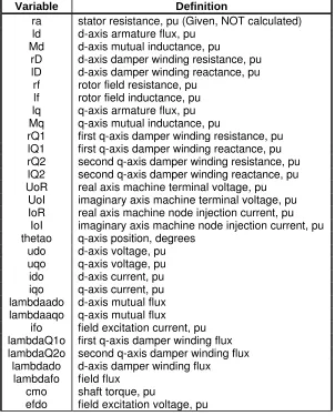
Table A.1: Coefficient Expansion Variable Definitions

ra

stator resistance, pu (Given, NOT calculated)

ld

d-axis armature flux, pu

Md

d-axis mutual inductance, pu

rD

d-axis damper winding resistance, pu

lD

d-axis damper winding reactance, pu

rf

rotor field resistance, pu

lf

rotor field inductance, pu

lq

q-axis armature flux, pu

Mq

q-axis mutual inductance, pu

rQ1

first q-axis damper winding resistance, pu

lQ1

first q-axis damper winding reactance, pu

rQ2

second q-axis damper winding resistance, pu

lQ2

second q-axis damper winding reactance, pu

UoR

real axis machine terminal voltage, pu

UoI

imaginary axis machine terminal voltage, pu

IoR

real axis machine node injection current, pu

IoI

imaginary axis machine node injection current, pu

thetao

q-axis position, degrees

udo

d-axis voltage, pu

uqo

q-axis voltage, pu

ido

d-axis current, pu

iqo

q-axis current, pu

lambdaado

d-axis mutual flux

lambdaaqo

q-axis mutual flux

ifo

field excitation current, pu

lambdaQ1o

first q-axis damper winding flux

lambdaQ2o

second q-axis damper winding flux

lambdado

d-axis damper winding flux

lambdafo

field flux

cmo

shaft torque, pu

A

PPENDIX

B

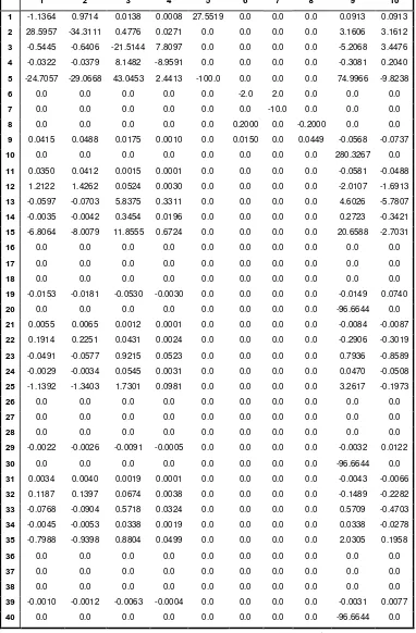
A-matrix Coefficients, Base Case

[image:10.612.116.498.96.678.2]

Table B.1: Columns 1-10 of State Matrix A

1 -1.1364 0.9714 0.0138 0.0008 27.5519 0.0 0.0 0.0 0.0913 0.0913 2 28.5957 -34.3111 0.4776 0.0271 0.0 0.0 0.0 0.0 3.1606 3.1612 3 -0.5445 -0.6406 -21.5144 7.8097 0.0 0.0 0.0 0.0 -5.2068 3.4476 4 -0.0322 -0.0379 8.1482 -8.9591 0.0 0.0 0.0 0.0 -0.3081 0.2040 5 -24.7057 -29.0668 43.0453 2.4413 -100.0 0.0 0.0 0.0 74.9966 -9.8238

6 0.0 0.0 0.0 0.0 0.0 -2.0 2.0 0.0 0.0 0.0

7 0.0 0.0 0.0 0.0 0.0 0.0 -10.0 0.0 0.0 0.0 8 0.0 0.0 0.0 0.0 0.0 0.2000 0.0 -0.2000 0.0 0.0 9 0.0415 0.0488 0.0175 0.0010 0.0 0.0150 0.0 0.0449 -0.0568 -0.0737 10 0.0 0.0 0.0 0.0 0.0 0.0 0.0 0.0 280.3267 0.0 11 0.0350 0.0412 0.0015 0.0001 0.0 0.0 0.0 0.0 -0.0581 -0.0488 12 1.2122 1.4262 0.0524 0.0030 0.0 0.0 0.0 0.0 -2.0107 -1.6913 13 -0.0597 -0.0703 5.8375 0.3311 0.0 0.0 0.0 0.0 4.6026 -5.7807 14 -0.0035 -0.0042 0.3454 0.0196 0.0 0.0 0.0 0.0 0.2723 -0.3421 15 -6.8064 -8.0079 11.8555 0.6724 0.0 0.0 0.0 0.0 20.6588 -2.7031

16 0.0 0.0 0.0 0.0 0.0 0.0 0.0 0.0 0.0 0.0

17 0.0 0.0 0.0 0.0 0.0 0.0 0.0 0.0 0.0 0.0

18 0.0 0.0 0.0 0.0 0.0 0.0 0.0 0.0 0.0 0.0

19 -0.0153 -0.0181 -0.0530 -0.0030 0.0 0.0 0.0 0.0 -0.0149 0.0740 20 0.0 0.0 0.0 0.0 0.0 0.0 0.0 0.0 -96.6644 0.0 21 0.0055 0.0065 0.0012 0.0001 0.0 0.0 0.0 0.0 -0.0084 -0.0087 22 0.1914 0.2251 0.0431 0.0024 0.0 0.0 0.0 0.0 -0.2906 -0.3019 23 -0.0491 -0.0577 0.9215 0.0523 0.0 0.0 0.0 0.0 0.7936 -0.8589 24 -0.0029 -0.0034 0.0545 0.0031 0.0 0.0 0.0 0.0 0.0470 -0.0508 25 -1.1392 -1.3403 1.7301 0.0981 0.0 0.0 0.0 0.0 3.2617 -0.1973

26 0.0 0.0 0.0 0.0 0.0 0.0 0.0 0.0 0.0 0.0

27 0.0 0.0 0.0 0.0 0.0 0.0 0.0 0.0 0.0 0.0

28 0.0 0.0 0.0 0.0 0.0 0.0 0.0 0.0 0.0 0.0

29 -0.0022 -0.0026 -0.0091 -0.0005 0.0 0.0 0.0 0.0 -0.0032 0.0122 30 0.0 0.0 0.0 0.0 0.0 0.0 0.0 0.0 -96.6644 0.0 31 0.0034 0.0040 0.0019 0.0001 0.0 0.0 0.0 0.0 -0.0043 -0.0066 32 0.1187 0.1397 0.0674 0.0038 0.0 0.0 0.0 0.0 -0.1489 -0.2282 33 -0.0768 -0.0904 0.5718 0.0324 0.0 0.0 0.0 0.0 0.5709 -0.4703 34 -0.0045 -0.0053 0.0338 0.0019 0.0 0.0 0.0 0.0 0.0338 -0.0278 35 -0.7988 -0.9398 0.8804 0.0499 0.0 0.0 0.0 0.0 2.0305 0.1958

36 0.0 0.0 0.0 0.0 0.0 0.0 0.0 0.0 0.0 0.0

37 0.0 0.0 0.0 0.0 0.0 0.0 0.0 0.0 0.0 0.0

38 0.0 0.0 0.0 0.0 0.0 0.0 0.0 0.0 0.0 0.0

[image:11.612.123.491.100.677.2]

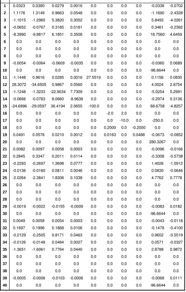
Table B.2: Columns 11-20 of State Matrix A

11 12 13 14 15 16 17 18 19 20

1 0.0323 0.0380 0.0279 0.0016 0.0 0.0 0.0 0.0 -0.0338 -0.0702 2 1.1176 1.3149 0.9663 0.0548 0.0 0.0 0.0 0.0 -1.1690 -2.4328 3 -1.1015 -1.2960 5.3820 0.3052 0.0 0.0 0.0 0.0 5.8493 -4.0261 4 -0.0652 -0.0767 0.3185 0.0181 0.0 0.0 0.0 0.0 0.3461 -0.2382 5 -8.3990 -9.8817 6.1851 0.3508 0.0 0.0 0.0 0.0 18.7560 4.6459

6 0.0 0.0 0.0 0.0 0.0 0.0 0.0 0.0 0.0 0.0

7 0.0 0.0 0.0 0.0 0.0 0.0 0.0 0.0 0.0 0.0

8 0.0 0.0 0.0 0.0 0.0 0.0 0.0 0.0 0.0 0.0

9 -0.0054 -0.0064 -0.0609 -0.0035 0.0 0.0 0.0 0.0 -0.0360 0.0689 10 0.0 0.0 0.0 0.0 0.0 0.0 0.0 0.0 -96.6644 0.0 11 -1.1448 0.9616 0.0285 0.0016 27.5519 0.0 0.0 0.0 0.1156 0.0830 12 28.3072 -34.6505 0.9867 0.0560 0.0 0.0 0.0 0.0 4.0024 2.8754 13 -1.1248 -1.3233 -22.9034 7.7309 0.0 0.0 0.0 0.0 -5.0254 5.2991 14 -0.0666 -0.0783 8.0660 -8.9638 0.0 0.0 0.0 0.0 -0.2974 0.3136 15 -24.6996 -29.0597 36.4194 2.0655 -100.0 0.0 0.0 0.0 68.6758 -4.8257

16 0.0 0.0 0.0 0.0 0.0 -2.0 2.0 0.0 0.0 0.0

17 0.0 0.0 0.0 0.0 0.0 0.0 -10.0 0.0 -250.0 0.0 18 0.0 0.0 0.0 0.0 0.0 0.2000 0.0 -0.2000 0.0 0.0 19 0.0491 0.0578 0.0210 0.0012 0.0 0.0163 0.0 0.0488 -0.0673 -0.0852 20 0.0 0.0 0.0 0.0 0.0 0.0 0.0 0.0 280.3267 0.0 21 0.0082 0.0097 0.0058 0.0003 0.0 0.0 0.0 0.0 -0.0096 -0.0166 22 0.2845 0.3347 0.2011 0.0114 0.0 0.0 0.0 0.0 -0.3308 -0.5738 23 -0.2293 -0.2697 1.3698 0.0777 0.0 0.0 0.0 0.0 1.4026 -1.0912 24 -0.0136 -0.0160 0.0811 0.0046 0.0 0.0 0.0 0.0 0.0830 -0.0646 25 -2.0264 -2.3841 1.8306 0.1038 0.0 0.0 0.0 0.0 4.7762 0.7778

26 0.0 0.0 0.0 0.0 0.0 0.0 0.0 0.0 0.0 0.0

27 0.0 0.0 0.0 0.0 0.0 0.0 0.0 0.0 0.0 0.0

28 0.0 0.0 0.0 0.0 0.0 0.0 0.0 0.0 0.0 0.0

29 -0.0019 -0.0022 -0.0155 -0.0009 0.0 0.0 0.0 0.0 -0.0083 0.0182 30 0.0 0.0 0.0 0.0 0.0 0.0 0.0 0.0 -96.6644 0.0 31 0.0049 0.0058 0.0054 0.0003 0.0 0.0 0.0 0.0 -0.0043 -0.0118 32 0.1697 0.1996 0.1868 0.0106 0.0 0.0 0.0 0.0 -0.1478 -0.4100 33 -0.2129 -0.2505 0.8171 0.0463 0.0 0.0 0.0 0.0 0.9652 -0.5519 34 -0.0126 -0.0148 0.0484 0.0027 0.0 0.0 0.0 0.0 0.0571 -0.0327 35 -1.3651 -1.6061 0.7764 0.0440 0.0 0.0 0.0 0.0 2.8788 0.9872

36 0.0 0.0 0.0 0.0 0.0 0.0 0.0 0.0 0.0 0.0

37 0.0 0.0 0.0 0.0 0.0 0.0 0.0 0.0 0.0 0.0

38 0.0 0.0 0.0 0.0 0.0 0.0 0.0 0.0 0.0 0.0

[image:12.612.120.494.99.678.2]

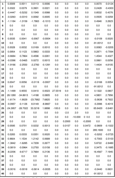
Table B.3: Columns 21-30 of State Matrix A

1 0.0009 0.0011 0.0113 0.0006 0.0 0.0 0.0 0.0 0.0070 -0.0124 2 0.0322 0.0379 0.3901 0.0221 0.0 0.0 0.0 0.0 0.2428 -0.4303 3 -0.4447 -0.5232 0.1549 0.0088 0.0 0.0 0.0 0.0 0.8532 0.4376 4 -0.0263 -0.0310 0.0092 0.0005 0.0 0.0 0.0 0.0 0.0505 0.0259 5 -1.1184 -1.3159 -1.7863 -0.1013 0.0 0.0 0.0 0.0 0.4946 3.2623

6 0.0 0.0 0.0 0.0 0.0 0.0 0.0 0.0 0.0 0.0

7 0.0 0.0 0.0 0.0 0.0 0.0 0.0 0.0 0.0 0.0

8 0.0 0.0 0.0 0.0 0.0 0.0 0.0 0.0 0.0 0.0

9 0.0035 0.0041 -0.0067 -0.0004 0.0 0.0 0.0 0.0 -0.0109 0.0020 10 0.0 0.0 0.0 0.0 0.0 0.0 0.0 0.0 -91.8312 0.0 11 0.0028 0.0032 0.0169 0.0010 0.0 0.0 0.0 0.0 0.0083 -0.0205 12 0.0954 0.1123 0.5863 0.0333 0.0 0.0 0.0 0.0 0.2871 -0.7094 13 -0.6684 -0.7864 0.4596 0.0261 0.0 0.0 0.0 0.0 1.4544 0.4327 14 -0.0396 -0.0465 0.0272 0.0015 0.0 0.0 0.0 0.0 0.0861 0.0256 15 -1.9166 -2.2550 -2.2760 -0.1291 0.0 0.0 0.0 0.0 1.4434 4.8105

16 0.0 0.0 0.0 0.0 0.0 0.0 0.0 0.0 0.0 0.0

17 0.0 0.0 0.0 0.0 0.0 0.0 0.0 0.0 0.0 0.0

18 0.0 0.0 0.0 0.0 0.0 0.0 0.0 0.0 0.0 0.0

19 0.0047 0.0056 -0.0118 -0.0007 0.0 0.0 0.0 0.0 -0.0168 0.0054 20 0.0 0.0 0.0 0.0 0.0 0.0 0.0 0.0 -91.8312 0.0 21 -1.1499 0.9555 0.0410 0.0023 27.5519 0.0 0.0 0.0 0.1322 0.0807 22 28.1280 -34.8613 1.4188 0.0805 0.0 0.0 0.0 0.0 4.5801 2.7956 23 -1.6174 -1.9029 -23.7662 7.6820 0.0 0.0 0.0 0.0 -5.0638 6.7922 24 -0.0957 -0.1126 8.0149 -8.9667 0.0 0.0 0.0 0.0 -0.2996 0.4019 25 -24.3957 -28.7022 33.3218 1.8898 -100.0 0.0 0.0 0.0 65.6420 -0.6461

26 0.0 0.0 0.0 0.0 0.0 -2.0 2.0 0.0 0.0 0.0

27 0.0 0.0 0.0 0.0 0.0 0.0 -10.000 0 0.0 0.0 0.0 28 0.0 0.0 0.0 0.0 0.0 0.2000 0.0 -0.2000 0.0 0.0 29 0.0595 0.0701 0.0232 0.0013 0.0 0.0157 0.0 0.0472 -0.0809 -0.1022 30 0.0 0.0 0.0 0.0 0.0 0.0 0.0 0.0 285.1600 0.0 31 0.0283 0.0333 0.0351 0.0020 0.0 0.0 0.0 0.0 -0.0202 -0.0725 32 0.9804 1.1534 1.2142 0.0689 0.0 0.0 0.0 0.0 -0.7003 -2.5103 33 -1.3842 -1.6285 4.7209 0.2677 0.0 0.0 0.0 0.0 5.8722 -2.8480 34 -0.0819 -0.0964 0.2793 0.0158 0.0 0.0 0.0 0.0 0.3475 -0.1685 35 -8.2206 -9.6717 3.7664 0.2136 0.0 0.0 0.0 0.0 16.4567 7.1945

36 0.0 0.0 0.0 0.0 0.0 0.0 0.0 0.0 0.0 0.0

37 0.0 0.0 0.0 0.0 0.0 0.0 0.0 0.0 0.0 0.0

38 0.0 0.0 0.0 0.0 0.0 0.0 0.0 0.0 0.0 0.0

[image:13.612.121.493.99.678.2]

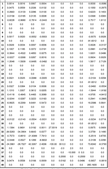
Table B.4: Columns 31-40 of State Matrix A

31 32 33 34 35 36 37 38 39 40

1 0.0014 0.0016 0.0067 0.0004 0.0 0.0 0.0 0.0 0.0030 -0.0086 2 0.0475 0.0559 0.2336 0.0132 0.0 0.0 0.0 0.0 0.1050 -0.2975 3 -0.2663 -0.3133 0.2286 0.0130 0.0 0.0 0.0 0.0 0.6223 0.1403 4 -0.0158 -0.0185 0.0135 0.0008 0.0 0.0 0.0 0.0 0.0368 0.0083 5 -0.8228 -0.9680 -0.7814 -0.0443 0.0 0.0 0.0 0.0 0.7517 1.9112

6 0.0 0.0 0.0 0.0 0.0 0.0 0.0 0.0 0.0 0.0

7 0.0 0.0 0.0 0.0 0.0 0.0 0.0 0.0 0.0 0.0

8 0.0 0.0 0.0 0.0 0.0 0.0 0.0 0.0 0.0 0.0

9 0.0017 0.0020 -0.0052 -0.0003 0.0 0.0 0.0 0.0 -0.0070 0.0028 10 0.0 0.0 0.0 0.0 0.0 0.0 0.0 0.0 -91.8312 0.0 11 0.0029 0.0034 0.0097 0.0006 0.0 0.0 0.0 0.0 0.0028 -0.0137 12 0.1007 0.1185 0.3372 0.0191 0.0 0.0 0.0 0.0 0.0981 -0.4738 13 -0.3844 -0.4522 0.4850 0.0275 0.0 0.0 0.0 0.0 1.0201 0.0486 14 -0.0227 -0.0268 0.0287 0.0016 0.0 0.0 0.0 0.0 0.0604 0.0029 15 -1.3548 -1.5939 -0.8495 -0.0482 0.0 0.0 0.0 0.0 1.5817 2.7129

16 0.0 0.0 0.0 0.0 0.0 0.0 0.0 0.0 0.0 0.0

17 0.0 0.0 0.0 0.0 0.0 0.0 0.0 0.0 0.0 0.0

18 0.0 0.0 0.0 0.0 0.0 0.0 0.0 0.0 0.0 0.0

19 0.0021 0.0025 -0.0088 -0.0005 0.0 0.0 0.0 0.0 -0.0104 0.0058 20 0.0 0.0 0.0 0.0 0.0 0.0 0.0 0.0 -91.8312 0.0 21 0.0327 0.0384 0.0104 0.0006 0.0 0.0 0.0 0.0 -0.0460 -0.0554 22 1.1310 1.3307 0.3612 0.0205 0.0 0.0 0.0 0.0 -1.5944 -1.9192 23 -0.4118 -0.4845 5.4465 0.3089 0.0 0.0 0.0 0.0 4.9705 -4.8412 24 -0.0244 -0.0287 0.3223 0.0183 0.0 0.0 0.0 0.0 0.2941 -0.2865 25 -6.9925 -8.2269 9.6491 0.5472 0.0 0.0 0.0 0.0 19.2086 0.0641

26 0.0 0.0 0.0 0.0 0.0 0.0 0.0 0.0 0.0 0.0

27 0.0 0.0 0.0 0.0 0.0 0.0 0.0 0.0 0.0 0.0

28 0.0 0.0 0.0 0.0 0.0 0.0 0.0 0.0 0.0 0.0

29 -0.0122 -0.0143 -0.0554 -0.0031 0.0 0.0 0.0 0.0 -0.0234 0.0718 30 0.0 0.0 0.0 0.0 0.0 0.0 0.0 0.0 -91.8312 0.0 31 -1.1384 0.9691 0.0192 0.0011 27.5519 0.0 0.0 0.0 0.0975 0.0909 32 28.5283 -34.3904 0.6643 0.0377 0.0 0.0 0.0 0.0 3.3759 3.1490 33 -0.7573 -0.8910 -21.8389 7.7913 0.0 0.0 0.0 0.0 -5.2519 3.8705 34 -0.0448 -0.0527 8.1289 -8.9602 0.0 0.0 0.0 0.0 -0.3108 0.2290 35 -24.3961 -28.7027 42.3267 2.4006 -100.00 00 0.0 0.0 0.0 73.8342 -8.3793

36 0.0 0.0 0.0 0.0 0.0 -2.0 2.0 0.0 0.0 0.0

A

PPENDIX

C

MATLAB Source Code

C.1

initcond.m

% % % This program calculates the initial conditions: % % % % UoR real axis machine terminal voltage, pu % % UoI imaginary axis machine terminal voltage, pu % % IoR real axis machine node injection current, pu % % IoI imaginary axis machine node injection current, pu % % thetao q-axis position, degrees % % udo d-axis voltage, pu % % uqo q-axis voltage, pu % % ido d-axis current, pu % % iqo q-axis current, pu % % lambdaado d-axis mutual flux % % lambdaaqo q-axis mutual flux % % ifo field excitation current, pu % % lambdaQ1o first q-axis damper winding flux % % lambdaQ2o second q-axis damper winding flux % % lambdado d-axis damper winding flux % % lambdafo field flux % % cmo shaft torque, pu % % efdo field excitation voltage, pu % % % %%%%%%%%%%%%%%%%%%%%%%%%%%%%%%%%%%%%%%%%%%%%%%%%%%%%%%%%%%%%%%%%%%%%%%%%%%%%%%%%

% Start of Program ---%

%%%%%%%%%%%%%%%%%%%%%%%%%%%%%%%%%%%%%%%%%%%%%%%%%%%%%%%%%%%%%%%%%%%%%%%%%%%%%%%% % Part One % % Eurostag Machine Parameter Conversion - External to Internal % %%%%%%%%%%%%%%%%%%%%%%%%%%%%%%%%%%%%%%%%%%%%%%%%%%%%%%%%%%%%%%%%%%%%%%%%%%%%%%%%

% Input Values ---% % Machine Parameters (External)

Xd = 1.8; Xpd = 0.3; Xppd = 0.25; Xq = 1.7; Xpq = 0.55; Xppq = 0.25; ra = 0.0025; Xl = 0.2; Tpdo = 8.0; Tppdo = 0.03; Tpqo = 0.4; Tppqo = 0.05;

inputd = [Xd Xpd Xppd Tpdo Tppdo]; inputq = [Xq Xpq Xppq Tpqo Tppqo]; inputmut = [ra Xl];

%---End of Parameter Input %

% Eurostag 4-winding calculations ---%

% d-axis values ---%

omegao = 120*pi; Tpd = Xpd*(Tpdo/Xd); Tppd = Xppd*(Tppdo/Xpd);

dB1 = (Tpdo + Tppdo)*omegao; dB2 = (Tpd + Tppd)*omegao;

dC1 = (Tpdo*Tppdo)*(omegao*omegao); dC2 = (Tpd*Tppd)*(omegao*omegao);

ld = Xl; Md = Xd - Xl;

dQ = (1/dX) - (1/Md); dB = dC2 - dC1*(ld/Xd);

dRAD = sqrt(1 - (4*dB*ld*dQ*dQ)/(dX*dP*dP));

dV1 = (-0.5*dP*(1+dRAD))/dQ; dV2 = (-0.5*dP*(1-dRAD))/dQ; dV = [dV1; dV2];

dU1 = (dB*ld)/(dX*dV1); dU2 = (dB*ld)/(dX*dV2); dU = [dU1; dU2];

dZ1 = (dB*ld) + (Md*dV1)*(dB2+(dP/dQ)); dZ2 = (dB*ld) + (Md*dV2)*(dB2+(dP/dQ));

dE1 = (dC1 - (dZ1/dX))/(Md*(dU1-dV1)); dE2 = (dC1 - (dZ2/dX))/(Md*(dU2-dV2)); dE = [dE1; dE2];

drf1 = 1/dE1; drf2 = 1/dE2; drf = [drf1; drf2];

dalf = (Tpd*Md - Tpdo*dX)/(Tpdo-Tpd); darf = (Md+dalf)/(Tpdo*omegao);

% selection of rf value

dummyd1 = abs(darf-drf1); dummyd2 = abs(darf-drf2); if dummyd1 < dummyd2

selectiond = 1; else

selectiond = 2; end

dF = ((dB2+(dP/dQ))/dX) - (dE(selectiond)); rD = 1/dF;

lD = rD*(dU(selectiond)); rf = drf(selectiond); lf = rf*(dV(selectiond));

% d-axis output

outputd = [Md ld rf lf rD lD];

%---End of d-axis calculations %

% q-axis values ---%

Tpq = Xpq*(Tpqo/Xq); Tppq = Xppq*(Tppqo/Xpq);

qB1 = (Tpqo + Tppqo)*omegao; qB2 = (Tpq + Tppq)*omegao;

qC1 = (Tpqo*Tppqo)*(omegao*omegao); qC2 = (Tpq*Tppq)*(omegao*omegao);

lq = Xl; Mq = Xq - Xl;

qX = (Mq*lq)/Xq;

qP = (qB1/Mq) - (qB2/qX); qQ = (1/qX) - (1/Mq); qB = qC2 - qC1*(lq/Xq);

qRAD = sqrt(1 - (4*qB*lq*qQ*qQ)/(qX*qP*qP));

qU1 = (qB*lq)/(qX*qV1); qU2 = (qB*lq)/(qX*qV2); qU = [qU1; qU2];

qZ1 = (qB*lq) + (Mq*qV1)*(qB2+(qP/qQ)); qZ2 = (qB*lq) + (Mq*qV2)*(qB2+(qP/qQ));

qE1 = (qC1 - (qZ1/qX))/(Mq*(qU1-qV1)); qE2 = (qC1 - (qZ2/qX))/(Mq*(qU2-qV2)); qE = [qE1; qE2];

qrQ1 = 1/qE1; qrQ2 = 1/qE2; qrQ = [qrQ1; qrQ2];

qalQ1 = (Tpq*Mq - Tpqo*qX)/(Tpqo-Tpq); qarQ1 = (Mq+qalQ1)/(Tpqo*omegao);

% selection of rQ value

dummyq1 = abs(qarQ1-qrQ1); dummyq2 = abs(qarQ1-qrQ2); if dummyq1 < dummyq2

selectionq = 1; else

selectionq = 2; end

qF = ((qB2+(qP/qQ))/qX) - (qE(selectionq)); rQ2 = 1/qF;

lQ2 = rQ2*(qU(selectionq)); rQ1 = qrQ(selectionq); lQ1 = rQ1*(qV(selectionq));

% q-axis output

outputq = [Mq lq rQ1 lQ1 rQ2 lQ2];

%---End of q-axis calculations %

%---End of External Value to Internal Value Conversion %

%%%%%%%%%%%%%%%%%%%%%%%%%%%%%%%%%%%%%%%%%%%%%%%%%%%%%%%%%%%%%%%%%%%%%%%%%%%%%%%% % Part Two % % Eurostag Initial Conditions Calculation % %%%%%%%%%%%%%%%%%%%%%%%%%%%%%%%%%%%%%%%%%%%%%%%%%%%%%%%%%%%%%%%%%%%%%%%%%%%%%%%%

% Input Values ---% % From Load Flow

UN = 20.0; PN = 800.0; SN = 900.0;

Polf = 700.0; Qolf = 400.0; Ulf = 20.0; theta = 25.0;

Po = Polf/SN; Qo = Qolf/SN; U = Ulf/UN;

%---End of Load Flow Values Input %

% Initial Conditions Calculation ---%

% machine terminal voltage

% machine node injection current

IoR = (Po*UoR + Qo*UoI) / (UoR*UoR + UoI*UoI); IoI = (Po*UoI - Qo*UoR) / (UoR*UoR + UoI*UoI);

% q-axis position

thetao = atan((UoI+omegao*(Mq+lq)*IoR+ra*IoI)/(UoR+ra*IoR-omegao*(Mq+lq)*IoI));

% Park voltages and currents

udo = (UoR*sin(thetao)) - (UoI*cos(thetao)); uqo = (UoR*cos(thetao)) + (UoI*cos(thetao));

ido = ((IoR*sin(thetao)) - (IoI*cos(thetao)))*(100/SN); iqo = ((IoR*sin(thetao)) + (IoI*cos(thetao)))*(100/SN);

% mutual fluxes

lambdaado = (-1.0/omegao)*(uqo + ra*iqo + omegao*ld*ido); lambdaaqo = (-1.0/omegao)*(udo + ra*ido - omegao*lq*iqo);

% field excitation current

ifo = (lambdaado/Md) - ido;

% winding fluxes

lambdaQ1o = lambdaaqo; lambdaQ2o = lambdaQ1o; lambdado = lambdaado + ifo;

lambdafo = (lambdaado + (lf*ifo));

% shaft torque

cmo = ((-lambdaado*iqo) + (lambdaaqo*ido))*(100/SN);

% field excitation voltage

efdo = -Md*ifo;

%---End of Initial Values Calculations %

%---End of Program %

C.2

matrixab.m

%%%%%%%%%%%%%%%%%%%%%%%%%%%%%%%%%%%%%%%%%%%%%%%%%%%%%%%%%%%%%%%%%%%%%%%%%%%%%%%% % % % File Name: matrixab.m % % % % Purpose: Calculate Eurostag A and B Matrix coefficients from machine % % data and load flow initial conditions parameters % % % % Follows: initcond.m, using the output variables of: % % % % ra stator resistance, pu (Given, NOT calculated) % % ld d-axis armature flux, pu % % Md d-axis mutual inductance, pu % % rD d-axis damper winding resistance, pu % % lD d-axis damper winding reactance, pu % % rf rotor field resistance, pu % % lf rotor field inductance, pu % % lq q-axis armature flux, pu % % Mq q-axis mutual inductance, pu % % rQ1 first q-axis damper winding resistance, pu % % lQ1 first q-axis damper winding reactance, pu % % rQ2 second q-axis damper winding resistance, pu % % lQ2 second q-axis damper winding reactance, pu % % UoR real axis machine terminal voltage, pu % % UoI imaginary axis machine terminal voltage, pu % % IoR real axis machine node injection current, pu % % IoI imaginary axis machine node injection current, pu % % thetao q-axis position, degrees % % udo d-axis voltage, pu % % uqo q-axis voltage, pu % % ido d-axis current, pu % % iqo q-axis current, pu % % lambdaado d-axis mutual flux % % lambdaaqo q-axis mutual flux % % ifo field excitation current, pu % % lambdaQ1o first q-axis damper winding flux % % lambdaQ2o second q-axis damper winding flux % % lambdado d-axis damper winding flux % % lambdafo field flux % % cmo shaft torque, pu % % efdo field excitation voltage, pu % % % % Notes: % % % % Uses differential and algebraic state equation derivation from % % Eurostag V2.3 theory manual % % % % System in the form of DXdot = A DX + B DU, with DXdot consisting of: % % omega % % theta % % lambdaf % % lambdad % % lambdaQ1 % % lambdaQ2 % % % %%%%%%%%%%%%%%%%%%%%%%%%%%%%%%%%%%%%%%%%%%%%%%%%%%%%%%%%%%%%%%%%%%%%%%%%%%%%%%%%

% Start of Program ---%

% Initialization of Variables ---%

% Initial Frequency

freqo = 60.0;

% Temporary Variable Calculation

LppMD = (1/Md) + (1/lf) + (1/lD); LppMD = 1/LppMD;

LpMQ = (1/Mq) + (1/lQ1) + (1/lQ2); LpMQ = 1/LpMQ;

r2denom = (ra*ra) + (lq + LpMQ)*(ld + LppMD); Lnumer = LpMQ - LppMD + lq - ld;

%---End of Variable Initialization %

% A Matrix Coefficients ---%

% The partial of d/dt(omega) with respect to each of the variables, row one

A11 = 0;

dIQtheta =

((ra*UoR*sin(thetao))-(ra*UoI*cos(thetao))+((ld+LppMD)*UoR*cos(thetao))+((ld+LppMD)*UoI*sin(thetao)))/(r2denom); dIDtheta = ((-ra*UoI*sin(thetao))-(ra*UoR*cos(thetao))+((lq+LpMQ)*UoR*sin(thetao))-((lq+LpMQ)*UoI*cos(thetao)))/(r2denom);

A12 = ((LppMD)/(2*H*lf))*lambdafo*dIQtheta + ((LppMD)/(2*H*lD))*lambdado*dIQtheta ((LpMQ)/(2*H*lQ1))*lambdaQ1o*dIDtheta ((LpMQ)/(2*H*lQ2))*lambdaQ2o*dIDtheta -((Lnumer)/(2*H))*ido*dIQtheta - ((Lnumer)/(2*H))*iqo*dIDtheta;

dIQf = (-ra*(LppMD/lf))/(r2denom); dIDf = ((lq+LpMQ)*(LppMD/lf))/(r2denom);

A13 = ((LppMD)/(2*H*lf))*iqo + ((LppMD)/(2*H*lf))*lambdafo*dIQf + ((LppMD)/(2*H*lD))*lambdado*dIQf + ((LpMQ)/(2*H*lQ1))*lambdaQ1o*dIDf +

((LpMQ)/(2*H*lQ2))*lambdaQ2o*dIDf - ((Lnumer)/(2*H))*ido*dIQf - ((Lnumer)/(2*H))*iqo*dIDf;

dIQd = (-ra*(LppMD/lD))/(r2denom); dIDd = ((lq+LpMQ)*(LppMD/lD))/(r2denom);

A14 = ((LppMD)/(2*H*lf))*lambdafo*dIQd + ((LppMD)/(2*H*lD))*iqo + ((LppMD)/(2*H*lD))*lambdado*dIQd + ((LpMQ)/(2*H*lQ1))*lambdaQ1o*dIDd +

((LpMQ)/(2*H*lQ2))*lambdaQ2o*dIDd - ((Lnumer)/(2*H))*ido*dIQd - ((Lnumer)/(2*H))*iqo*dIDd;

dIQQ1 = (-(ld+LppMD)*(LpMQ/lQ1))/(r2denom); dIDQ1 = (ra*(LpMQ/lQ1))/(r2denom);

A15 = ((LppMD)/(2*H*lf))*lambdafo*dIQQ1 + ((LppMD)/(2*H*lD))*lambdado*dIQQ1

-((LpMQ)/(2*H*lQ1))*ido - ((LpMQ)/(2*H*lQ1))*lambdaQ1o*dIDQ1 - ((LpMQ)/(2*H*lQ2))*lambdaQ2o*dIDQ1 - ((Lnumer)/(2*H))*ido*dIQQ1 - ((Lnumer)/(2*H))*iqo*dIDQ1;

dIQQ2 = (-(ld+LppMD)*(LpMQ/lQ2))/(r2denom); dIDQ2 = (ra*(LpMQ/lQ2))/(r2denom);

A16 = ((LppMD)/(2*H*lf))*lambdafo*dIQQ2 + ((LppMD)/(2*H*lD))*lambdado*dIQQ2

-((LpMQ)/(2*H*lQ1))*lambdaQ1o*dIDQ2 - ((LpMQ)/(2*H*lQ2))*ido - ((LpMQ)/(2*H*lQ2))*lambdaQ2o*dIDQ2 - ((Lnumer)/(2*H))*ido*dIQQ2 - ((Lnumer)/(2*H))*iqo*dIDQ2;

%---End of row one %

% The partial of d/dt(theta) with respect to each of the variables, row two

A21 = omegao; A22 = 0.0; A23 = 0.0; A24 = 0.0; A25 = 0.0; A26 = 0.0;

%---End of row two %

omo = 2*freqo*pi;

A31 = 0.0;

prelf = (omo*rf*LppMD)/lf;

A32 = prelf*dIDtheta;

A33 = -((omo*rf)/lf) + ((omo*rf*LppMD)/(lf*lf)) - prelf*dIDf;

A34 = ((omo*rf*LppMD)/(lf*lD)) - prelf*dIDd;

A35 = prelf*dIDQ1;

A36 = prelf*dIDQ2;

%---End of row 3 %

% The partial of d/dt(lambdad) with respect to each of the variables, row 4

A41 = 0.0;

prelD = (omo*rD*LppMD)/lD;

A42 = prelD*dIDtheta;

A43 = ((omo*rD*LppMD)/(lf*lD)) - prelD*dIDf;

A44 = ((omo*rD*LppMD)/(lD*lD)) - ((omo*rD)/lD) - prelD*dIDd;

A45 = prelD*dIDQ1;

A46 = prelD*dIDQ2;

%---End of row 4 %

% The partial of d/dt(lambdaQ1) with respect to each of the variables, row 5

A51 = 0.0;

prelQ1 = (omo*rQ1*LpMQ)/(lQ1);

A52 = prelQ1*dIQtheta;

A53 = prelQ1*dIQf;

A54 = prelQ1*dIQd;

A55 = ((omo*rQ1*LpMQ)/(lQ1*lQ1)) - ((omo*rQ1)/lQ1) - prelQ1*(-dIQQ1);

A56 = ((omo*rQ1*LpMQ)/(lQ1*lQ2)) - prelQ1*(-dIQQ2);

%---End of row 5 %

% The partial of d/dt(lambdaQ2) with respect to each of the variables, row 6

A61 = 0.0;

prelQ2 = (omo*rQ2*LpMQ)/(lQ2);

A62 = prelQ2*dIQtheta;

A63 = prelQ2*dIQf;

A64 = prelQ2*dIQd;

A65 = ((omo*rQ2*LpMQ)/(lQ1*lQ2)) - prelQ2*(-dIQQ1);

%---End of A Matrix Coefficient Calculation %

% B Matrix Coefficients ---%

B11 = (PN/200*H)*cmo; B12 = 0.0;

B21 = 0.0; B22 = 0.0;

B31 = 0.0;

B32 = -(omo*rf)/Md;

B41 = 0.0; B42 = 0.0;

B51 = 0.0; B52 = 0.0;

B61 = 0.0; B62 = 0.0;

%---End of B Matrix Coefficient Calculation %

% Matrix Formulation ---%

MatrixA = [A11 A12 A13 A14 A15 A16 A21 A22 A23 A24 A25 A26 A31 A32 A33 A34 A35 A36 A41 A42 A43 A44 A45 A46 A51 A52 A53 A54 A55 A56 A61 A62 A63 A64 A65 A66];

MatrixB = [B11 B12 B21 B22 B31 B32 B41 B42 B51 B52 B61 B62];

NDIFF = 6;

%---End of Matrix Formulation %

%---End of Program %

C.3

eigval.m

%%%%%%%%%%%%%%%%%%%%%%%%%%%%%%%%%%%%%%%%%%%%%%%%%%%%%%%%%%%%%%%%%%%%%%%%%%%%%%%% % % % Filename: eigval.m % % % % Purpose: Eigenvalues, Frequency, Damping, Left and Right Eigenvector % % and Participation Factor calculation for a given a Matrix % % % % Follows: matrixab.m % % % % Variable Name Definition % % --- --- % % MatrixA A Matrix from matrixab.m % % REV Right Eigenvector % % LEV Scaled Left Eigenvector % % eigenvalue(i) Column Vector of i Eigenvalues (Eval) % % wdn(i) Damped Natural Frequency of ith Eval, rad/sec % % fdn(i) Damped Natural Frequency of ith Eval, Hz % % damping(i) Damping Coefficient of ith eval % % PF(i,j) Participation Factor, REV*LEV % % MODE(i) Oscillatory Modes % % PFMODE(i,j) Participation Factor of Mode(i) % % % %%%%%%%%%%%%%%%%%%%%%%%%%%%%%%%%%%%%%%%%%%%%%%%%%%%%%%%%%%%%%%%%%%%%%%%%%%%%%%%%

% Start of Program---%

% Eigenvalue and Right Eigenvector Calculation ---%

[REV,EVR] = eig(MatrixA);

% [REV,EVR] = eig(FULL_ARED) returns the matrices EVR and REV where % EVR is a diagonal matrix of the eigenvalues of FULL_ARED and % REV is a full matrix whose columns are the corresponding % right eigenvectors so that FULL_ARED * REV = REV * EVR

eigenvalue = diag(EVR);

% "eigenvalue" is a column vector containing the eigenvalues

%---Matlab Default Function, Left Eigenvector not Normalized---% %[LEV,EVL] = eig(FULL_ARED');

%LEV = LEV'; %

% Creates diagonal matrix EVL of eigenvalues and a full matrix

% LEV whose columns are the corresponding left eigenvectors satisfying % LEV * FULL_ARED = EVL * LEV

% The eigenvalues in EVR and EVL are the same, but not in the same order %---%

% Normalized Left Eigenvector Calculation ---%

LEV=inv(REV);

%---End of Eigenvector Calcualtion %

% Participation Factor Calculation ---%

% Note: NOT for each Mode, but for each Eigenvalue

for i = 1:NDIFF

for j = 1:NDIFF

PF(i,j) = REV(i,j) * LEV(j,i); end

end

% q = left eigenvector)

% Oscillatory Mode Participation Factor Calculation ---%

% Eliminate the conjugate eigenvalues and calculate the participation % factor associated with each mode of oscillation

%

% LOOP allows the elimination of the conjugate eigenvalues % (The complex conjugate existing in "eigenvalue") %

% OSC = number of oscillatory modes %

% MODE = vector with one eigenvalue associated with each oscillatory

% mode

%

% PFMODE = matrix with the participation factor of each oscillatory mode

LOOP=0; OSC=1;

for i=1:NDIFF-1

if LOOP == 0 % do not eliminate the eigenvalue

if abs(imag(eigenvalue(i))) > 0

% complex eigenvalue

if (eigenvalue(i) == conj(eigenvalue(i+1))) % conjugate eigenvalue MODE(OSC)=eigenvalue(i); for j=1:NDIFF

PFMODE(j,OSC)=PF(j,i)+PF(j,i+1); % sum of the two participation factors % of the two eigenvalues

end LOOP=1;

% allow the elimination of the conjugate % during the next iteration

end

else % real eigenvalue case

MODE(OSC)=eigenvalue(i); for j=1:NDIFF

PFMODE(j,OSC)=PF(j,i); end

end OSC=OSC+1; else

LOOP=0; end

end OSC=OSC-1;

%---End of Participation Factor Calculation %

% Results Output ---%

% Save Participation Factors in the file "eigvalpf.afs"

% lines = oscillatory modes

% colomns = state variables

fid = fopen('eigvalpf.afs','w'); i=0;

fprintf(fid,'%8.4f',i); for i=1:NDIFF

fprintf(fid,'%8.4f',i); end

fprintf(fid,'\n');

for i=1:OSC

fprintf(fid,'%8.4f',PFMODE(j,i)); end

fprintf(fid,'\n'); end

fclose(fid);

% Save the eigenvalues, oscillation frequency and damping in the file % "eigvaldamp.afs"

fid = fopen('eigvaldamp.afs','w'); for i=1:OSC

wdn(i)=abs(imag(MODE(i))); sgma(i)=real(MODE(i)); fdn(i)=wdn(i)/(2*pi);

damping(i)=-sgma(i)/sqrt(sgma(i)*sgma(i)+wdn(i)*wdn(i));

% wdn(i) = oscillation corresponding to each (eigenvalue) MODE(i) % sgma(i) = real part of each MODE(i)

% fdn(i) = frequency of the oscillatory mode of each (eigenvalue) MODE(i) % damping(i) = damping coefficient corresponding to each (eigenvalue) % MODE(i)

fprintf(fid,'%8.0f %10.4f %10.4f %10.4f %10.4f\n',i, sgma(i), imag(MODE(i)), fdn(i), damping(i));

end

%---End of Results Output %

%---End of Program %

C.4

eigalyze.m

%%%%%%%%%%%%%%%%%%%%%%%%%%%%%%%%%%%%%%%%%%%%%%%%%%%%%%%%%%%%%%%%%%%%%%%%%%%%%%%% % % % Filename: eigalyze.m % % % % Purpose: Eigenvalues, Frequency, Damping, Left and Right Eigenvector % % and Participation Factor calculation for the Eurostag- % % provided state-space system % % % % Variable Name Definition % % --- --- % % ARED Reduced A Matrix % % REV Right Eigenvector % % LEV Scaled Left Eigenvector % % eigenvalue(i) Column Vector of i Eigenvalues (Eval) % % wdn(i) Damped Natural Frequency of ith Eval, rad/sec % % fdn(i) Damped Natural Frequency of ith Eval, Hz % % damping(i) Damping Coefficient of ith eval % % PF(i,j) Participation Factor, REV*LEV % % MODE(i) Oscillatory Modes % % PFMODE(i,j) Participation Factor of Mode(i) % % % %%%%%%%%%%%%%%%%%%%%%%%%%%%%%%%%%%%%%%%%%%%%%%%%%%%%%%%%%%%%%%%%%%%%%%%%%%%%%%%% % % % Eurostag Interface Notes: % % % % Using the Eurostag algebraic-differential state equations, % % the state equations are linearized, yielding the system % % % % Xdot = f(X,Y) -> xdot = f0 + Mx + Ny % % 0 = g(X,Y) -> 0 = g0 + Px + Qy % % % % where x = X - X0 % % y = Y - Y0 % % f0 = f(X0, Y0) % % g0 = g(X0, Y0) % % % % The linearized system information from Eurostag is available in three % % different file types: % % .linear ASCII file with all variables % % .lineared ASCII file, algebraic equations are eliminated % % .mat Matlab readable file % % % % The .linear and .mat files contain the following: % % % % NDIFF = Number of differential variables (dimension X) % % NVAR = Total number of variables (differential and algebraic, % % dimension X + Y) % % A matrix = | M N | = sparse matrix formed by I J A(I,J) % % | P Q | % % V0 vector = | X0 | % % | Y0 | % % F0 vector = | f0 | % % | g0 | % % % % The .lineared file contains the same information except that the % % matrix ARED = M-N*invQ*P is created in lieu of the matrix A. % % % % The information derived from the .linear, .lineared and .mat files % % is complemented by another ASCII file, .keylin, which contains the % % information for the differential state equations and their % % corresponding macroblocks. % % % %%%%%%%%%%%%%%%%%%%%%%%%%%%%%%%%%%%%%%%%%%%%%%%%%%%%%%%%%%%%%%%%%%%%%%%%%%%%%%%%

% Reduced A Matrix Construction ---%

load 1pmu_gen212.mat

% Load "filename.mat" (must be changed for each case)

% Eurostag V2.4 output file containing linearized state variable data

NDIM = NVAR;

% NDIM = Total number of variables

jaco = sparse(I,J,A);

% sparse - Builds sparse matrix jaco (Jacobian) with matrix % coefficient A(i) at the Jth column and the Ith row

% Matrix A Sub-Matrix Formation ---%

M = jaco(1:NDIFF,1:NDIFF); N = jaco(1:NDIFF,NDIFF+1:NDIM); P = jaco(NDIFF+1:NDIM,1:NDIFF); Q = jaco(NDIFF+1:NDIM,NDIFF+1:NDIM);

% Sparse sub-matrices M, N, P and Q built from Jacobian matrix

% Reduced A Matrix Calculation ---%

ARED = (M-N*inv(Q)*P);

% Reduced A matrix calculation (ARED) = elimination of the algebraic % state variables

FULL_ARED = full(ARED);

% FULL - Conversion of "sparse" matrix ARED into "full" matrix FULL_ARED

%---End of A Matrix Construction %

% Eigenvalue and Right Eigenvector Calculation ---%

[REV,EVR] = eig(FULL_ARED);

% [REV,EVR] = eig(FULL_ARED) returns the matrices EVR and REV where % EVR is a diagonal matrix of the eigenvalues of FULL_ARED and % REV is a full matrix whose columns are the corresponding % right eigenvectors so that FULL_ARED * REV = REV * EVR

for i=1:NDIFF

for j=1:NDIFF

rrev(i,j) = real(REV(i,j)); irev(i,j) = imag(REV(i,j)); end

end

eigenvalue = diag(EVR);

% "eigenvalue" is a column vector containing the eigenvalues

%---Matlab Default Function, Left Eigenvector not Normalized---% %[LEV,EVL] = eig(FULL_ARED');

%LEV = LEV'; %

% Creates diagonal matrix EVL of eigenvalues and a full matrix

% LEV whose columns are the corresponding left eigenvectors satisfying % LEV * FULL_ARED = EVL * LEV

% The eigenvalues in EVR and EVL are the same, but not in the same order %---%

%---End of Eigenvector Calcualtion %

% Participation Factor Calculation ---%

% Note: NOT for each Mode, but for each Eigenvalue

for i = 1:NDIFF

for j = 1:NDIFF

PF(i,j) = abs(REV(i,j) * LEV(j,i)); end

end

% Calculates the participation factors, dimensionless measures of the % state xk in mode i (Pki = pki * qki, p = right eigenvector,

% q = left eigenvector). Returns the magnitude of the complex number, % the value of interest (Kundur, p. 777)

% Oscillatory Mode Participation Factor Calculation ---%

% Eliminate the conjugate eigenvalues and calculate the participation % factor associated with each mode of oscillation

%

% LOOP allows the elimination of the conjugate eigenvalues % (The complex conjugate existing in "eigenvalue") %

% OSC = number of oscillatory modes %

% MODE = vector with one eigenvalue associated with each oscillatory

% mode

%

% PFMODE = matrix with the participation factor of each oscillatory mode

LOOP=0; OSC=1;

for i=1:NDIFF-1

if LOOP == 0 % do not eliminate the eigenvalue

if abs(imag(eigenvalue(i))) > 0

% complex eigenvalue

if (eigenvalue(i) == conj(eigenvalue(i+1))) % conjugate eigenvalue MODE(OSC)=eigenvalue(i); for j=1:NDIFF

PFMODE(j,OSC)=PF(j,i)+PF(j,i+1); % sum of the two participation factors % of the two eigenvalues

end LOOP=1;

% allow the elimination of the conjugate % during the next iteration

end

else % real eigenvalue case

MODE(OSC)=eigenvalue(i); for j=1:NDIFF

PFMODE(j,OSC)=PF(j,i); end

end OSC=OSC+1; else

LOOP=0; end

end OSC=OSC-1;

%---End of Participation Factor Calculation %

% Save the Eigenvalues in: % "FILENAME-eig.afs"

fid = fopen('1pmu_gen212-eig.afs','w'); for i=1:NDIFF

re(i) = real(eigenvalue(i)); ie(i) = imag(eigenvalue(i));

fprintf(fid,'%8.0f %11.5f %11.5f\n', i, re(i), ie(i)); end

% Save the Modes, Oscillation Frequency and Damping in: % "FILENAME-frdm.afs"

fid = fopen('1pmu_gen212-frdm.afs','w'); for i=1:OSC

wdn(i)=abs(imag(MODE(i))); sgma(i)=real(MODE(i)); fdn(i)=wdn(i)/(2*pi);

damping(i)=-sgma(i)/sqrt(sgma(i)*sgma(i)+wdn(i)*wdn(i));

% wdn(i) = oscillation corresponding to each (eigenvalue) MODE(i) % sgma(i) = real part of each MODE(i)

% fdn(i) = frequency of the oscillatory mode of each (eigenvalue) MODE(i) % damping(i) = damping coefficient corresponding to each (eigenvalue) % MODE(i)

fprintf(fid,'%8.0f %10.4f %10.4f %10.4f %10.4f\n',i, sgma(i), imag(MODE(i)), fdn(i), damping(i));

end

% Save Right Eigenvectors in: % "FILENAME-rev.afs"

% columns = vector corresponding to each eigenvalue

fid = fopen('1pmu_gen212-rev.afs','w');

for i=1:NDIFF

fprintf(fid,'%8.4f',i); for j=1:NDIFF

fprintf(fid,'%8.4f %8.4f',rrev(j,i),irev(j,i)); end

fprintf(fid,'\n'); end

fclose(fid);

% Save Participation Factors in: % "FILENAME-pf.afs"

% lines = oscillatory modes

% columns = state variables

fid = fopen('1pmu_gen212-pf.afs','w'); i=0;

fprintf(fid,'%8.4f',i); for i=1:NDIFF

fprintf(fid,'%8.4f',i); end

fprintf(fid,'\n');

for i=1:OSC

fprintf(fid,'%8.4f',i); for j=1:NDIFF

fprintf(fid,'%8.4f',PFMODE(j,i)); end

fprintf(fid,'\n'); end

fclose(fid);

V

ITA

Aaron F. Snyder was born in Parkersburg, West Virginia, and graduated from Parkersburg South

High School in 1988. He attended Virginia Polytechnic Institute and State University (Virginia

Tech) in Blacksburg, Virginia, where he obtained his Bachelor of Science in Electrical

Engineering degree in 1993, with minors in math and music. He then decided to continue his

studies at Virginia Tech, returning in the fall of 1993 as a Master of Science candidate in electrical

engineering. To pursue his interest in music, he auditioned to enter into the music program at

Virginia Tech, and was accepted in the spring of 1994 as a candidate for the Bachelor of Arts in

Music Performance.

At the end of his coursework for his master's degree, he applied for and was accepted as the first

student in an exchange program between Virginia Tech and the

Institut National Polytechnique

de Grenoble

(I.N.P.G.) in Grenoble, France. Through this program, he completed a

Diplôme

d’Etudes Approfondies

(master’s equivalent degree) in June 1996 at I.N.P.G. He is currently a

Doctorat de l’I.N.P.G.

(Ph.D.) candidate in electrical engineering at I.N.P.G.