THE IMPACT OF MACROECONOMIC VARIABLES TOWARD CREDIT DEFAULT SWAP SPREADS IN ASIA AND EUROPE
Created by:
RIZMA YANIKA CHUSNA 1110081100018
MANAGEMENT DEPARTMENT INTERNATIONAL PROGRAM
FACULTY OF ECONOMIC AND BUSINESS
v
CURRICULUM VITAE
Personal Identities
Name : Rizma Yanika Chusna Gender : Female
Place of Birth : Curup
Date of Birth : January, 12th 1992
Address : Kemang Ifi Graha blok F9/14, Jati Asih, Bekasi. Phone/Mobile : 085966656322
E-mail Address : [email protected]
Formal Education
College : UIN Syarif Hidayatullah Jakarta Senior High School : SMAN 48 Jakarta
Junior High School : SMPN 9 Bekasi
vi
ABSTRACT
This study empirically examines the impact of the interaction between macroeconomic variables and the Credit Default Swap (CDS) spreads with 5 years maturity in Asia and Europe. The applied macroeconomic variables in this research are: GDP growth, inflation, unemployment, import/GDP, and current account balance. This study uses annually data from 2009-2013. Using panel data regression method with the Random Effect Model, the finding can be summarized as follows: (i) the inflation, unemployment, and current account balance variable is significantly affect the CDS spreads in Asia and Europe , while the GDP growth and import/GDP are not significantly affect the CDS spreads in Asia and Europe. (ii) inflation and unemployment have positive sign, indicates that the higher inflation and unemployment leads to the higher Credit Default Swap spreads, meanwhile, current account balance has a negative sign, indicates that the higher current account balance leads to the lower Credit Default Swap spreads. (iii) Based on the research, the result shows that 26.42% of the independent variables have influence the dependent variable that is the Credit Default Swap spreads, while the rest of 73.58% influenced by the other variables which are not contained in this research.
vii
ABSTRAK
Penelitian ini secara empiris bertujuan untuk menguji dampak dari interaksi antara variabel ekonomi makro dan Credit Default Swap (CDS) Spreads dengan 5 tenor tahun di Asia dan Eropa. Variabel makroekonomi yang digunakan dalam penelitian ini adalah: pertumbuhan PDB, inflasi, pengangguran, impor/GDP, dan neraca transaksi berjalan. Penelitian ini menggunakan data tahunan pada periode 2009-2013. Dengan menggunakan metode regresi data panel dengan Random Effect Model, hasil dari temuan dapat dijabarkan sebagai berikut: (i) variabel inflasi, pengangguran, dan neraca transaksi berjalan secara signifikan mempengaruhi CDS spreads di Asia dan Eropa, sedangkan variabel pertumbuhan PDB dan impor / GDP tidak berpengaruh secara signifikan terhadap CDS spreads di Asia dan Eropa. (ii) variabel inflasi dan pengangguran memiliki tanda positif, mendandakan bahwa peningkatan tingkat inflasi dan pengangguran menyebabkan peningkatan pada Credit Default Swap spreads, sementara itu, neraca transaksi berjalan memiliki tanda negatif, mendandakan bahwa peningkatan pada neraca transaksi berjalan menyebabkan penurunan pada Credit Default Swap spreads. (iii) Hasil dari penelitian menunjukkan bahwa sebesar 26.42% variabel independen dapat menjelaskan variabel dependen yaitu Credit Default Swap spreads, sedangkan sisanya 73.58% dijelaskan oleh variabel-variabel lain yang tidak terdapat dalam penelitian.
viii
PREFACE Assalamu’alaikum Wr. Wb.
All praise to Allah SWT, because of His blessings and grace the writer can finish this thesis as one of the requirements in accomplishing the bachelor degree.
The writer also want to thank profusely to all of the parties who had sacrificing their time to give motivation and advice to the writer, thus, this thesis can be finished properly. The writer realizes that without the support from the several parties, this thesis cannot be finished properly. In this change, the writer would like to say thank to:
1. My Parents Achmad Chusnun and Ratna Sari, who always support me morally and materially. Thank you for always encourage me to finish my thesis. Thank you for your love and always pray for your daughter. Sorry I have not been able to repay all that you give for me on the last 22 years. 2. Prof. Dr. Abdul Hamid, MS., as the Dean of Economic and Business Faculty
UIN Syarif Hidayatullah.
3. Prof. Dr. Ahmad Rodoni as my supervisor I, who always encourage, guide and motivate me. Thank you for the time that you have spared to help me to finish this thesis. Thank you for always being nice when I ask question sir. May Allah gives His blessing for you.
4. Titi Dewi Warninda, SE., M.Si as my supervisor II, who always encourage, guide and motivate me. Thank you for the time that you have spared to help me to finish this thesis. May Allah gives His blessing for you.
ix
6. Pak Raffi and his friends from “Biro Kebijakan Fiskal” Indonesian Ministry
of Finance, who also help me in data collection process. Thank you so much, without your help, this thesis cannot be complete.
7. All of the staff in Economic and Business Faculty on 3rd floors. Especially pak Bonyx who always nicely help me to prepare the documents that I need to make the thesis.
8. Elfa Halim Ahmad and Annisa Gustiarawanti who always support me and accompany me in order to get the data that I need to finish this thesis. Sometimes we are fight, sometime we are arguing, sometimes we are dissent, sometimes we are complaining about one and each other. Nevertheless, behind that, there were million of memorable moments that we have passed together. You are all the best that I ever had. Thank you for all joy and the sorrow that all we share together for the last 4 years.
9. My friends in Management International 2010 who always nice to me: Afif, Andro, Rahim, Erbi, Ali, Aufa, Futri and Diena. Thank you for being good friends.
10.Little brother Muhammad Rizal Fahim who always support me.
11.All of the friends who always help me during the assistance Shelly, Anjar, Aris, Vae, and Umi
The writer realizes that this thesis is far from perfection due to the limited knowledge of writer. All of the suggestions and criticism are welcomed in order to make this thesis better. I hope, this thesis will be useful for the other researcher or reader.
Jakarta, November ,2014 The Writer
x
TABLE OF CONTENT
Curriculum Vitae ... v
Abstract ... vi
Abstrak ... vii
Preface ... viii
Table of Contents ... x
List of Tables... xiv
List of Figures ... xv
List of Appendix ... xvi
Chapter I INTRODUCTION A. Background ... 1
B. Formulation of the Problem ... 9
C. Research Purposes ... 9
D. Research Advantages ... 10
Chapter II LITERTURE REVIEW A. Bond ... 11
1. Characteristic of Bond... 12
2. Bond Pricing... 12
B. Credit Ratings... 13
C. Credit Risk and Credit Default ... 15
D. Credit Default Swap ... 16
xi
E. Macroeconomic Variables ... 20
1. GDP Growth Rate ... 21
2. Inflation ... 22
3. Unemployment ... 23
4. Import/GDP ... 24
5. Current Account Balance ... 25
F. Previous Research ... 26
G. Theoretical Framework... 31
H. Hypothesis ... 33
Chapter III RESEARCH METHODOLOGY A. Scope of the Research ... 36
B. Sampling Method ... 36
C. Data Collection Method ... 37
D. Analysis Technique ... 38
1. Analysis Method ... 38
2. Stationary Test ... 38
3. Classic Assumption Test ... 39
a. Normality Test ... 39
b. Heteroscedasticity Test ... 40
c. Multicollinearity Test... 41
d. Autocorrelation Test... 42
4. Panel Data Regression ... 42
a. Pooled Ordinary Least Square (PLS) ... 44
xii
c. Random Effect Model (REM) ... 46
(1) Model Selection on Panel Data ... 47
(a) Chow Test ... 47
(b) Hausman Test... 48
5. t-test ... 49
6. F-test ... 49
7. Adjusted R2 ... 50
E. Variable Operational Research ... 50
1. Independent Variables ... 50
a. GDP Growth... 50
b. Inflation ... 50
c. Unemployment ... 51
d. Import/GDP ... 51
e. Current Account Balance ... 51
2. Dependent Variable ... 51
Chapter IV FINDING AND ANALYSIS A. General Description of Research Object ... 53
1. Credit Default Swap ... 54
2. Bloomberg LP ... 55
B. Data Description ... 56
1. Descriptive Statistics ... 56
a. CDS Spreads ... 57
b. GDP Growth... 57
c. Inflation ... 57
xiii
e. Import/GDP ... 57
f. Current account balance ... 58
2. Data Processing ... 66
a. Stationary Test ... 66
b. Classic Assumption Test ... 69
(1) Normality Test... 69
(2) Heteroscedasticy Test... 71
(3) Multicollinearity Test ... 72
(4) Autocorrelation Test... 73
c. Model Selection in Panel Data Regression... 74
(1) Chow Test ... 75
(2) Hausman Test ... 76
d. Hypothesis Testing ... 77
(1) t-Test ... 77
(2) F-Test ... 82
e. Regression Equation... 83
f. The Effect of Macroeconomic Variables in Explaining the Credit Default Swap spreads ... 85
Chapter V CONCLUSION A. Conclusion... 86
B. Suggestion ... 87
1. For Investors... 87
2. For Academics ... 88
xiv
C. The Limits of the Research and Recommendation ... 88
xv
LIST OF TABLES No. Description
1.1 Credit Ratings and Credit Default Swap Spread of Lehman Brothers ... 3
2.1 Definition of Bond Ratings Classification ... 14
2.2 Overview Previous Research ... 29
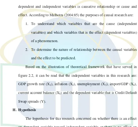
3.1 The Difference between Cross Section and Time Series Data ... 43
4.1 Descriptive Statistics ... 56
4.2 CDS Spreads ... 58
4.3 GDP Growth ... 59
4.4 Inflation ... 61
4.5 Unemployment Total ... 62
4.6 Import of Goods and Services/GDP ... 63
4.7 Current Account Balance ... 64
4.8 Stationary Test (at Level) ... 67
4.9 Stationary Test (at 1st Difference) ... 68
4.10 Stationary Test (at 2nd Difference) ... 69
4.11 The Result of White Heteroscedasticity Test ... 71
4.12 The Result of Multicollinearity Test ... 72
4.13 The Result of Autocorrelation Test using Durbin-Watson Statistic ... 73
4.14 The Result of Chow Test... 75
4.15 The Result of Hausman Test ... 76
4.16 The Result of t-Test ... 78
xvi
LIST OF FIGURES
No. Description
1.1 Asian CDS Spreads in Basis Points ... 5
2.1 Credit Default Swap Mechanism ... 18
2.2 Theoretical Framework ... 32
4.1 Annual CDS Notionals Outstanding ($) ... 54
xvii
LIST OF APPENDIX
No. Description
Appendix I List of Countries ... 94
Appendix II Descriptive Statistics ... 97
Appendix III Stationary Test ... 98
Appendix IV Normality Test ... 110
Appendix V Hesteroscedasticity Test ... 111
Appendix VI Multicollinearity Test ... 112
Appendix VII Autocorrelation Test... 113
Appendix VIII Chow Test ... 114
Appendix IX Hausman Test ... 115
Appendix X The Result of Pooled Least Square ... 116
Appendix XI The Result of Fixed Effect Model ... 117
Appendix XII The Result of Random Effect Model ... 118
Appendix XIII Partial t-Test ... 120
Appendix XIV Simultaneous F-Test ... 121
1
CHAPTER I
INTRODUCTION
A. Research Background
According to Fitch, credit ratings provide an opinion on the relative ability of an entity to meet financial commitments, such as interest, preferred dividends, re-payment of principal, insurance claims or counterparty obligations. Credit ratings have been used to measure the potential of default or default risk since long time ago. Default risk is the probability that the interest and principal will not be paid in the promised amounts on the due dates or will not be paid at all (Ross, et. al, 2010:628). Bond default risk or credit risk is measured by these global institutions, they are: εoody’s Investor Services, Standard & Poor Corporation (S&P), and Fitch Investors Service. These three institutions provide bond ratings on corporate or sovereign bond based on the evaluation of the probability that the bond issuer will make the promised payment.
In fact, there was a criticism on bond ratings or credit ratings during the global financial crisis led by the subprime mortgage crisis in 2008. During 2007-2008 credit ratings remained relatively unchanged. For example, California’s Orange County and Enron, received high credit ratings until just
2
of credit rating agency perform the accurate forecast during the subprime mortgage crisis led the investors to look for the other instruments that can accurately predict the bond investment.
In recent year, Credit Default Swap (CDS) assessed to be the more accurate predicted instrument rather than bond ratings. Credit Default Swap is an insurance contract which pays off in the event of credit event. Credit event mentioned here can be interpreted as default or bankruptcy (Keown, et. al, 2010:23). The credit default swap (CDS) is the most commonly-used credit derivative instrument, it has enabled investors to insure against a credit event such as the default of a reference entity. Reference entity mentioned here is the bond issuer (Baum and Wan, 2010). Sovereign Credit Default Swap (SCDS) can be used to protect investors against losses on sovereign debt arising from so-called credit events such as default or debt restructuring (IMF 2013). The buyers of CDS must pay the periodic premium or spread.
According to Flannery, et. al, (2010) even though the credit ratings remained relatively unchanged, CDS spreads increased during 2007 and 2008 as information became available showing that the probability of defaults by financial institutions was increasing. δehman Brother’s rating is still A until it
3
Table 1.1
Credit Ratings and Credit Default Swap Spread of Lehman Brothers
Date Lehman Brothers
Ratings Spread
1/2/06 A 25
1/1/07 A 21
4/2/07 A 38
7/10/07 A 45
8/17/07 A 150
1/1/08 A 120
3/14/08 A 448
9/12/08 A 702
9/15/08 A 703
Source: Sand, 2012
Table 1.1 shows that the Lehman Brothers ratings is still A even before it declare for it’s bankruptcy in September β008. According to εoody’s and
S&P, A rating means that the company has strong capacity to pay interest and principal. Based on the εoody’s and S&P description δehman Brothers is supposed to be far from bankrupt, because it has a strong capacity to pay interest and principle. In real, in September 2008, Lehman Brothers is declare for it bankruptcy. In the other hand, δehman Brothers’s Credit Default Swap
4
buyer and a seller of credit protection. The premium paid by the buyer of protection known as CDS spreads. CDS spreads change over time based on supply and demand for particular CDS contracts. In March 2008, Lehman Brothers spreads started to rise until September 2008. This trend was occurs due to the increasing on the CDS demand caused by the loss of investors confidence toward the δehman Brother’s future outlook. This was led by the subprime mortgage crisis where the Lehman Brother is contributed to sell the large number of subprime mortgage debenture. It proven that Credit Default Swap is more accurately in predicting the potential of default compare with the bond rating.
5
Figure 1.1
Asian CDS spread in basis points
Sources: Asian Development Bank (2012)
6
Furthermore, based on preceding illustration, the author is interested to figure out the relationship between macroeconomic variables and Credit Default Swap Spread in Asia and Europe. Because of that, “The Impact of
Macroeconomic Variables toward Credit Default Swap Spread in Asia and Europe” has been chosen by the author as the title of this research. For
conducting this research, the author uses some of macroeconomic variables. The macroeconomic variables that are used are: GDP growth rate, inflation, unemployment rate, import/GDP, and current account balance.
The author limits the sample into 9 Asian countries and 5 European countries. Asian countries are represented by: China, Hong Kong, Indonesia, Japan, Malaysia, Philippines, South Korea, Thailand, and Vietnam while European countries are represented by Germany, Ireland, Italy, Portugal, and Spain. The data that used by the author for conducting this research are the data from 2009-2013, in order to figure out the impact of macroeconomic variables on CDS spreads after global crisis or in the post global crisis.
7
shows that unemployment is the most significant variable, while inflation is the least significant variable that affecting CDS spread in PIIGS countries. Aini (2012) had conducted a research regarding the impact of interest rates, stock returns, and implied volatility toward Credit Default Swap spreads in Indonesia. In her research, Aini was employ government securities (SUN) with 10 years maturity as a proxy of interest rates, Jakarta Composite Index (JCI) returns as a proxy of stock returns, and vstoxx index as a proxy of implied volatility. This research uses multiple regression analysis as the method. The result shows that interest rates, stock returns and implied volatility have an impact toward Credit Default Swap spreads in Indonesia. Implied volatility has the most effect toward CDS spreads in Indonesia compare with the other independent variable.
8
CDS. The international reserve is the highest relatively to the two other coefficient. While, in the short-run, the external debt and international reserves are significant for eight emerging countries. The current account is not significant for all countries.
9
The researcher is using the countries that located in European contingen, because, it refers to the previous research that had been conducted by some of the researcher who is Brandorf and Holmberg (2010) and Sand (2012) that used some of European countries as a sample of their research. Meanwhile, in order to distinguish this research from the previous research, the researcher add the countries that located in Asia as a sample. In order to avoid the imbalances between Asian and European countries, thus, the researcher not only using the developing countries in Europe, but also the developed countries such as Portugal, Ireland, Italy, and Spain as the sample.
B. Formulation of the Problem
1. Is there any impact between GDP growth, inflation, unemployment, import/GDP, and current account balance partially toward the Credit Default Swap spreads in Asia and Europe?
2. Is there any effect between GDP growth, inflation, unemployment, import/GDP, and current account balance simultaneously toward the Credit Default Swap spreads in Asia and Europe?
C. Research Purposes
The purposes of this research are:
10
2. To examine empirically the effect of macroeconomic variables that represented by GDP growth, inflation, unemployment, import/GDP, and current account balance toward the Credit Default Swap spreads in Asia and Europe.
D. Research Advantages 1. For the Researcher
Enrich the author knowledge regarding the financial condition in Asia and Europe particularly on the derivatives market (bond and Credit Default Swap spread).
2. For the Investors
As a guidance for the investor who wants to particularly start their investing activity on sovereign bond to consider the macroeconomic condition that might affect bond market in a country before decides to do an investment. 3. For the Academics
a. Giving additional insight for the academics.
b. As a reference for the other researchers for conducting the research especially regarding Credit Default Swap spread.
4. For the Government
11
CHAPTER II LITERATURE REVIEW A. Bond
Bond is a security that is issued in connection with a borrowing agreement. Borrower (the issuer of the bond) sells a bond to the lender for some amount of cash. The agreement obligates the issuer to make specified payments to bond holder on specified dates. A typical coupon bond obligates the issuer to make semiannual payments of the interest to bondholder for the life of the bond (Bodie, et. al, 2009:446).
Bond is an instrument in which the issuer (borrower) promises to repay to the lender/investor the amount borrowed (principal) plus interest (coupon) over some specified period of time. The interest is usually paid at specified intervals, such as semi-annually or quarterly. When the bond matures, the investor receives the entire amount invested, or the principal plus coupon (www.idx.co.id, 2014a).
12
Bond is a long-term (10 years or more) promissory note issued by a borrower, promising to pay the owner of the security a predetermined amount of interest each year (Keown, et. al, 2011:27).
1. Characteristic of Bonds
According to www.idx.co.id (2014b), the characteristics of bond, are:
a. Nominal value (face value) is bond issued or bond principals.
b. Coupon (the interest rate) is the interest value occasionally received by the bondholders (usually every γ or 6 months). Bond’s coupon is asserted in
annual percentages.
c. Tenor (maturity) is the date when the bondholders will receive principal payment of the bond. The maturity date of each bond varies from 365 days to more than 5 years. A bond close to maturity date has lower risk than a bond that is far from maturity. It is because a bond that close to the maturity date is easier to predict.
2. Bond Pricing
13
a. Par Value = Bond’s price is the same as its nominal value.
For example: A bond with nominal value Rp 50 million sold at price 100%, the bond’s value is 100% x Rp 50 million = Rp 50
million.
b. At Premium = Bond’s price is higher than its nominal value.
For example: A bond with nominal value Rp 50 million sold at price 10β%, the bond’s value is 10β% x Rp 50 million = Rp 51
million.
c. At discount = Bond’s price is lower than its nominal value.
For example: Bond with nominal value Rp 50 million sold at price 98%, the bond’s value is 98% x Rp 50 million = Rp 49 million.
B. Credit Ratings
According to Fitch, credit ratings provide an opinion on the relative ability of an entity to meet financial commitments, such as interest, preferred dividends, repayment of principal, insurance claims or counterparty obligations.
According to S&P Credit ratings are forward-looking opinions about credit risk. Standard & Poor’s credit ratings express the agency’s opinion
14
Sovereign credit ratings are an assessment of the creditworthiness of a government’s ability and willingness to make timely payment of the principal and the interests of its debt (Mellios and Blanc, 2006).
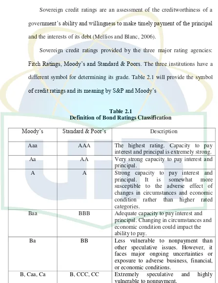
Sovereign credit ratings provided by the three major rating agencies: Fitch Ratings, εoody’s and Standard & Poors. The three institutions have a
[image:32.612.91.538.100.680.2]different symbol for determining its grade. Table 2.1 will provide the symbol of credit ratings and its meaning by S&P and εoody’s
Table 2.1
Definition of Bond Ratings Classification
εoody’s Standard & Poor’s Description
Aaa AAA The highest rating. Capacity to pay
interest and principal is extremely strong. Aa AA Very strong capacity to pay interest and
principal.
A A Strong capacity to pay interest and
principal. It is somewhat more susceptible to the adverse effect of changes in circumstances and economic condition rather than higher rated categories.
Baa BBB Adequate capacity to pay interest and
principal. Changing in circumstances and economic condition could impact the ability to pay.
Ba BB Less vulnerable to nonpayment than
other speculative issues. However, it faces major ongoing uncertainties or exposure to adverse business, financial, or economic conditions.
15
εoody’s Standard & Poor’s Description
C C No interest is being paid.
D D Default. Payments of interest or
repayment of principal is in arrears. Sources: Bodie, et. al (2009) and Keown, et. al (2011)
Although S&P and εoody’s have a different symbol for representing the investment grade, actually, the symbols have a similar meaning. BBB or above (S&P) or Baa and above (εoody’s) are considered as an investment-grade bonds, whereas lower-rated bonds are classified as speculative-investment-grade or junk bonds. (Bodie, et. al, 2009:467).
All rating agencies’ issuer credit ratings express a relative ranking of an issuer’s creditworthiness, which reflects the issuer's overall ability and
willingness to meet its senior, unsecured obligations. It is based on current information provided by obligors or obtained from other reliable sources. (Ismailescu and Kazemi, 2009).
C. Credit Risk and Credit Default
16
A sovereign default event occurs when a scheduled debt service is not paid in the specified in the debt contract. Unlike the corporation, on the rare occasion when the government defaults on its debt, it cannot declare for its bankruptcy. Under this situations, creditors and the defaulting borrower generally exchange or restructuring its debt (Ismailescu and Kazemi, 2009).
D. Credit Default Swap
Near the end of 20th century, a new derivatives instrument called Credit Default Swap (CDS) was emerge and introduced as a tools to measure the sovereign risk (Ariefianto and Soepomo, 2011).
A credit default swap is a bilateral agreement between two parties, a buyer and a seller of credit protection. In its simplest form, the protection buyer agrees to make periodic payments over a predetermined number of years (the maturity of the CDS) to the protection seller. In exchange, the protection seller commits to making a payment to the buyer in the event of default by a third party (the reference entity). CDS quotes now commonly relied upon as indicators of investor’s perceptions of credit risk regarding
17
One of the most important terms in a CDS agreement is the definition of a credit event. According to Fontana and Scheicher, 2010, the credit event described by International Swaps and Derivatives Association are (ISDA):
1. Failure to pay principal or coupon when they are due: the failure to pay a
coupon might represent a credit event, although most likely one with a high recovery.
2. Restructuring is a change in the terms of a debt obligation that is adverse
to creditors, such as a lengthening of the maturity of debt.
3. Repudiation / moratorium is occurs when the reference entity rejects or challenges the validity of its obligations.
There are some additional credit event added by Bomfim (2005:290) based on ISDA:
4. Bankruptcy is a situation where the reference entity unable to repay its
debts. This credit event does not apply to CDS written on sovereign reference entities.
5. Obligation Acceleration occurs when an obligation has become due and
payable earlier than it would have otherwise been.
18
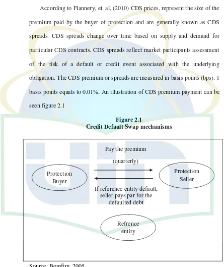
[image:36.612.91.536.104.633.2]According to Flannery, et. al, (2010) CDS prices, represent the size of the premium paid by the buyer of protection and are generally known as CDS spreads. CDS spreads change over time based on supply and demand for particular CDS contracts. CDS spreads reflect market participants assessment of the risk of a default or credit event associated with the underlying obligation. The CDS premium or spreads are measured in basis points (bps). 1 basis points equals to 0.01%. An illustration of CDS premium payment can be seen figure 2.1
Figure 2.1
Credit Default Swap mechanisms
Source: Bomfim, 2005
Generally the term of CDS have a similarity with the traditional insurance product. The protection buyers have to pay the premium or spreads
Protection Buyer
Protection Seller Pay the premium
(quarterly)
If reference entity default, seller pays par for the
defaulted debt
19
to the protection seller for secure their bond investment from the potential of default by the reference entity. If the reference entity facing the default during the life of the contract, the protection seller will pays the par to the protection buyers. Meanwhile, if the reference entity is not facing the default during the life of the contact, so that, the protection buyers will lose their premium or spread. Unlike the traditional insurance, should not to have any reference assets to buy the CDS. It generally called naked basis.
In the CDS spreads payment are known the terms of settlement payment. According to Carboni (2011), the settlement payment is made by the seller according to the contract settlement option. In credit derivatives, there are two options contract of the settlement, they are cash settlement and physical settlement.
20
1. The purposes of CDS
According to the types of reference entity, the CDS contracts can be categorized into two groups. The first one is corporate CDS and the other one is sovereign CDS. The International Monetary Fund (2013) is mentioned the objectives of Sovereign Credit Default Swap (SCDS):
a. Hedging : The owners of sovereign bond buy SCDS to protect
themselves against losses arising from a default or other credit event affecting the value of the underlying debt.
b. Speculating : SCDS contracts can be used to buy (or sell) protection on a naked basis, (the buyer of SCDS does not have any reference assets) to express a negative or positive opinion about the credit outlook of the issuer of the underlying bonds.
c. Basis trading : SCDS are used get a profit from differences between
SCDS and the underlying bond obligations price by taking offsetting positions in the two (“basis trading”). This strategy is based on the
principle that CDS can be used to replicate the cash flows of underlying obligations.
E. Macroeconomic Variables
21
emphasize on five macroeconomic variables to figure out the effect of macroeconomic variables toward CDS spreads in Asia and Europe. The following explanation will describe the macroeconomic variables used by the author:
1. GDP Growth Rate
Gross Domestic Product (GDP) is the total market value of all final goods and services produced within a given period by factors of production located within a country. (Case, et. al, 2009:129). Recent levels of country’s GDP may be used to measure recent economic growth
(Madura, 2010:480).
According to Frank and Bernanke (2009:439), there are two ways to measure GDP, they are:
a. Real GDP : a measure of GDP in which the quantities
produced are valued at the price in a base year rather than at current pricees; real GDP measures the actual physical volume of production.
22
the four components of GDP. The most important driver of GDP growth is personal consumption, which includes retail sales. GDP growth is also driven by business investment, which includes construction and inventory levels. Government spending is another driver of growth, and is sometimes necessary to jumpstart the economy after a recession. Last, but not least, are exports and imports. Exports drive growth, but increases in imports have a negative impact (Amadeo, 2014)
Annual percentage growth rate of GDP at market prices based on constant local currency. GDP is the sum of gross value added by all resident producers in the economy plus any product taxes and minus any subsidies not included in the value of the products. It is calculated without making deductions for depreciation of fabricated assets or for depletion and degradation of natural resources (www.worldbank.org, 2014a).
The research relates to the relationship between GDP growth and Credit Default Swap spreads had conducted by Brandrof and Homberlg (2010) indicate that CDS spreads decrease in GDP growth rate.
2. Inflation
23
According to www.worldbank.org (2014b), inflation can be determined by either Consumer Price Index or GDP deflator. Inflation as measured by the Consumer Price Index reflects the annual percentage change in the cost to the average consumer of acquiring a basket of goods and services. Meanwhile the inflation as measured by the annual growth rate of the GDP deflator shows the rate of price change in the economy as a whole. This research is using the inflation measured by the Consumer Price Index data.
The research relates to the relationship between inflation and the Credit Default Swap spreads had conducted by Sand (2012), the result indicates that the inflation variable is significantly affect the CDS spreads.
3. Unemployment
24
divided by the labor force. In general, a high rate of unemployment rate indicates that the economy of a country is performing poorly.
Unemployment rate is the ratio of the number of people employed to the total number of of people in the labor force (Case, et. al, 2009:148). Unemployment refers to the share of the labor force that is without work but available for and seeking for a job(www.worldbank.org, 2014c).
The research relates to the relationship between unemployment and Credit Default Swap spreads (CDS) had conducted by Brandrof and Holmberg (2010), the result shows that the CDS spreads increase in unemployment.
4. Import/GDP
Imports of goods and services represent the value of all goods and other market services received from the rest of the world. They include the value of merchandise, freight, insurance, transport, travel, royalties, license fees, and other services, such as communication, construction, financial, information, business, personal, and government services. They exclude compensation of employees and investment income (formerly called factor services) and transfer payments (www.worldbank.org,
25
The relationship between import/GDP and CDS spreads had conducted by Sand (2012), the result shows that the CDS spreads is increase along with the increasing on the import/GDP variable.
5. Current Account Balance
The balance of payments consist of the current account and capital account. In this study I focus on the current account. Current account represents a summary of the flow of funds between one specified country and all other countries due to the purchases of goods or services, or the provision of income on financial assets (Madura, 2010:27). Madura (2010:27-28) describes the main components of the current account, they are payments for:
a. Merchandise (goods and services) : merchandise exports and imports
represent tangible assets, while the service exports and imports represent tourism and other services, such as insurance.
b. Factor income payments : income (interest and dividend payments)
received by investors on foreign investment in financial assets.
c. Transfer payments : represented by aid and grants.
According to Case,et. al, (2009:402), the balance of payments is the record of a country’s transactions in goods, services, and assets with the
other countries, also the record of a country’s sources (supply) and uses
26
net exports of goods + net exports on services + net invetment income + net transfer payments.
The relationship between current account balance and Credit Default Swap spreads had conducted by Sand (2012), the result shows that the higher current account balance led to the lower CDS spreads.
F. Previous Research
Research regarding the effect of macroeconomic variables toward Credit Default Swap spread had conducted by some of the researchers. The result can be elaborated as follows:
1. Alexander and Andreas (β008) had conducted a research titled “Regime dependent determinants of credit default swap spreads”. In their research
Alexander used daily quotes of iTraxx Europe CDS indices and restrict the analysis to indices with a maturity of 5 years. The data period starts from June 2004 and ends in June 2007. The applied method for analyze are Linear regression and Markov switching regression. Using Interest rate, stock return and implied volatility variables, the result shows that All of the variables that is interest rate, stock return, and implied volatility are significant toward the CDS spreads.
2. Greatrex (2008) had conducted a research relates to the credit default swap market’s deteminants. In her research, Greatrex uses 333 firms as the sample
27
investigates the impact of these variables toward CDS spreads. The data for conducting this research is monthly, from January 2001 until March 2006. The result shows that a rating-based CDS index is the best predictor of CDS spread changes. Leverage and volatility, are also key determinants, as these two variables can explain almost half of the explained variation in monthly CDS spread changes.
3. Baum and Wan (2010) were conducted a research regarding the macroeconomic uncertainty and credit default swap spreads on individual firms. To measures the macroeconomic variables, Baum and Wan use variance of the GDP growth rate, the index of industrial production and the returns on the S&P 500 Composite Index and the other variables such as market value, leverage ratio, return on equity, and dividend payout ratio. For conducting this research, they used monthly data from January 2001 to December 2006, and 5 years CDS spreads from 527 firms. The result shows that the macroeconomic uncertainty is an important determinant of CDS spreads.
28
bond issuers denominated in US dollars with the period of outstanding CDS contracts between June 1997 and November 2006. They employ GDP growth rate, GDP growth volatility, jump risk and investor sentiment to measure the market conditions; and coefficient of variation in quarterly operating cash flow, firm growth, cash flow beta, leverage, implied volatility and jump (as the slope of option implied volatility curve) to measure the firm characteristics. The result shows that average credit spreads decrease in GDP growth rate, but increase in GDP growth volatility and jump risk in the equity market. At the market level, investor sentiment is the most important determinant of credit spreads. At the firm level, credit spreads generally rise with cash flow volatility and beta. Implied volatility is the most significant determinant of default risk among firm-level characteristics.
29
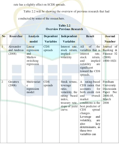
exchange rates has the most significant variable, while the domestic interest rate has a slightly effect on SCDS spreads.
[image:47.612.95.565.130.703.2]Table 2.2 will be showing the overview of previous research that had conducted by some of the researchers.
Table 2.2
Overview Previous Research No Resercher Analysis
model
Dependent Variables
Independent Variables
Result Journal
Number 1 Alexander
and Andreas (2008) Linear regression and Markov switching regression CDS spreads
Interest rate, stock return, implied volatility
All of the variables that is interest rate, stock return, and implied volatility are significant toward the CDS spreads.
Journal of Banking & Finance 32 (2008) 1008–1021
2 Greatrex (2008) Multivariat e regression model CDS spreads
Stock retuns, leverage ratio,
volatility, the rating based index,
treasury rate, slope of yield curve.
A rating-based CDS index that accounts for both credit risk and overall market
conditions is the best predictor of CDS spread changes.
Leverage and volatility, are
also key
30
No Researcher Analysis Model Dependent Variable Independent Variable Result explain almost half of the explained variation in monthly CDS spread changes.
Journal Number
3 Baum and Wan (2010) OLS and fixed-effect regression CDS spread Macroecono mic uncertainty (computed
by the
conditional variance of
the GDP
growth rate, the index of industrial production
and the
returns on the S&P 500 Composite Index.); market value; leverage ratio; ROE; Dividend payout ratio.
Macroeconomic uncertainty has significant explanatory power over and above that of traditional macroeconomic factors such as the risk-free rate and the Treasury term spread.
Applied Financial Economics Taylor & Francis Journal vol. 20 (15) page: 1163-1171
4 Tang and Yan (2010)
Regression Corporate credit spread
Firm CDS data; GDP growth rate; GDP growth volatility; Jump risk; Investor sentiment; CVCF; Firms
At the market level, investor sentiment is the most important determinant of credit spreads. At the firm level, credit spreads
Journal of Banking and
31
No Researcher Analysis Model
Dependent Variable
Independent Variable growth, Cash flow beta, Leverage, Implied volatility and Jump
Result
generally rise with cash flow volatility and beta. Implied volatility is the most significant determinant of default risk among firm-level
characteristics.
Journal Number
5 Liu and
Morley (2011)
VaR Sovereign
CDS spread
Domestic interest rates and
Exchange rates
Exchange rate has the most important effect on sovereign CDS markets.
Bath Economic Research Papers no 03/1, 2011.
Source: Author
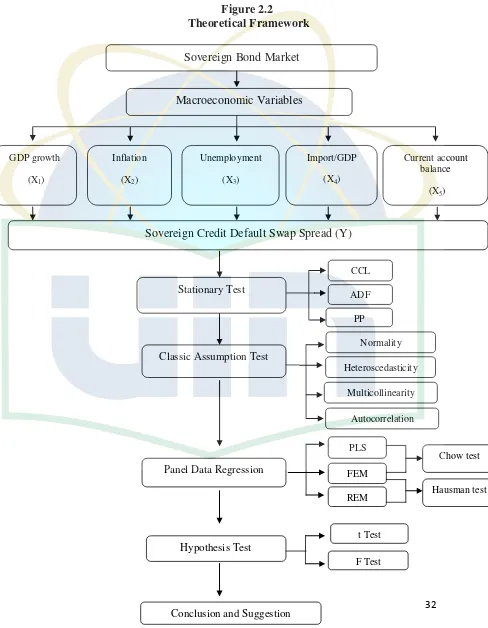
G. Theoretical Framework
32
Figure 2.2
Theoretical Framework
Sovereign Bond Market
Macroeconomic Variables GDP growth (X1) Inflation (X2) Unemployment (X3) Import/GDP (X4) Current account balance (X5)
Sovereign Credit Default Swap Spread (Y)
CCL
ADF
Classic Assumption Test
PLS FEM REM Hypothesis Test F Test t Test
Conclusion and Suggestion
PP Chow test Stationary Test Normality Heteroscedasticity Multicollinearity
Panel Data Regression
[image:50.612.91.579.111.739.2]33
The theoretical framework shows that the relationship between the dependent and independent variables is causative relationship or cause and effect. According to Malhotra (2004:85) the purposes of causal research are:
1. To understand which variables that are the cause (independent variables) and which variables that is the effect (dependent variables) of a phenomenon.
2. To determine the nature of relationship between the causal variables and the effect to be predicted.
Based on the illustration of theoretical framework that have served in figure 2.2, it can be read that the independent variables in this research are: GDP growth rate (X1), inflation (X2), unemployment (X3), import/GDP (X4), current account balance (X5) and the dependent variable that is Credit Default Swap spreads (Y).
H. Hypothesis
The hypothesis for this research concerned on whether there is an effect on dependent variable toward independent variable or there is no effect on dependent variable toward independent variable. Hypothesis of this research can be stated as follows:
[image:51.612.91.531.127.534.2]34
account balance toward Credit Default Swap spreads in Asia and Europe.
H1 = There are an effect between macroeconomic variables represented by GDP growth rate, inflation, unemployment, import/GDP, current account balance toward Credit Default Swap spreads in Asia and Europe.
2. H0 = GDP growth rate does not affect the Credit Default Swap spreads in Asia and Europe.
H1 = GDP growth rate does affect the Credit Default Swap spreads in Asia and Europe.
3. H0 = Inflation does not affect the Credit Default Swap spreads in Asia and Europe.
H1 = Inflation does affect the Credit Default Swap spreads in Asia and Europe.
4. H0 = Unemployment does not affect the Credit Default Swap spreads in Asia and Europe.
H1 = Unemployment does affect the Credit Default Swap spreads in Asia and Europe.
5. H0 = Import/GDP does not affect the Credit Default Swap spreads in Asia and Europe.
35
6. H0 = Current account balance does not affect the Credit Default Swap spreads in Asia and Europe.
36
CHAPTER III
RESEARCH METHODOLOGY
A. Scope of the Research
This research conducted by using eviews application and gretl to test the heteroscedasticity. Regression with the panel data used as a method of the research. This research emphasizes on 5 years maturity Credit Default Swap spreads in Asia and Europe at the time period of 2009-2013. The data that used by the author to conduct this research are secondary data, obtained from Bloomberg LP, www.worldbank.org, and www.quandl.com. The reason that makes the author select the period of 2009 until 2013 is to figure out the effect of macroeconomic variables toward CDS spreads after the global crisis.
B. Sampling Method
The sampling method used by the researcher in terms of conducting this research is judgment sampling or purposive sample. In this method, the data
are collected based on individual consideration. If the researcher convinces that the respondent is appropriate to be the object of the research, so that, the object can be chosen by the researcher for conducting the research.
Judgment sampling means that the sample is chosen based on the specific criteria in accordance with the purposes of the research. The criteria required to avoid the misspecification on determining the research’s sample which can
37
The sample of this research should have to meet the following criteria: 1. The countries located in Asian and European region.
2. Have a complete data that the author required. Such as have a complete GDP growth rate, inflation, unemployment, import/GDP, and current account balance data during the period of the research which is 2009 until 2013.
Based on the criteria described above, the samples that had chosen by the author for conducting this research are 9 Asian countries and 5 European countries. The selected Asian countries are China, Hong Kong, Indonesia, Japan, Malaysia, Philippines, South Korea, Thailand, and Vietnam, while the European countries are Germany, Ireland, Italy, Portugal, and Spain.
C. Data Collection Method
38
used for conducting this research is annually data from 2009-2013. The data for literature study is obtained from internet database, books, journals and other references.
D. Analysis Technique 1. Analysis Method
The researcher is using the panel data regression analysis to statistically test the hypothesis. Since, this research is types of causative research, so, the purpose of this research is to reveal the relationship between independent variable and dependent variable. Eviews program is used to know the result.
2. Stationary Test
Panel data that used in this research is the dynamic panel regression. In dynamic panel regression each variables requires stationary test. According to Granger and Newbold in Ariefianto (2012:124), the stationary test aimed to avoid the phenomena that known as spurious regression. Spurious or nonsense regression is a phenomena where a regression equation has a good siginificance (high R2) even though there is no meaningful relationship between the two variables (Gujarati, 2004:792). The hypothesis for stationary test is:
39
According to Gujarati (2004:815), we can reject the H0 of non-stationaryif the probability is < 0.05.
In this research, the stationary tested using Levin, Lin & Chu t, ADF, and PP unit root test. If the data is not stationer on the level, we can move
to the first difference or the second difference test.
3. Classic Assumption Test a. Normality Test
According to Gujarati (2004:147), there are three tests that can be used to detect the normality problem, they are: (1) histogram of residuals, (2) normal probability plot (NPP), (3) Jarque–Bera test. In eviews, the most commonly used test to detect the normality problem is Jarque–Bera test. The hypothesis for Jarque–Bera test for normality is:
H0 = residuals are normally distributed H1 = residuals are not normally distributed
40
b. Heteroscedasticity Test
If heteroscedasticity is detected in a regression model, thus the standard error from regression can be refraction (bias). As a consequences, all of the hypothesis test can be mislead. According to Ariefinto (2012:39) heteroscedasticity problem causes the conclution that concluded become invalid.
According to Fadhliyah (2008), there are several ways to detect the heteroscedasticity, it depends on the software used for conducting the research. In eviews, white heteroscedasticity is used to test the heteroscedasticity.
Beside eviews, the other application named gretl can be used to detect heteroscedasticity through white heteroscedasticity test.
The following hypothesis is built for heteroscedasticity test:
(1) H0 : Heteroscedasticity is not present (Homoscedastic) (2) H1 : Heteroscedastic
41
In gretl, the simplest way to tackle heteroscedasticity problem is to use least squares to estimate the intercept and slopes and use an estimator of least squares covariance that is consistent. This is the so-called heteroscedasticity robust estimator of covariance (Adkins, 2011:176).
Meanwhile, in eviews, Heteroscedasticity can be eliminated through White’s cross-section standard errors, if heteroscedasticity caused by the cross section or White’s period standard errors, if
heteroscedasticity caused by the variability over the time. If the heteroscedasticity caused by both cross section and time series, thus the it can eliminate through White’s diagonal standard errors.
c. Multicollinearity Test
The independent variables which contain of multicollinearity make the coefficient of regression become unsuitable with the substances, thus the interpretation become inappropriate (Fadhliyah, 2008).
According to (Wibowo, 2012: 87), one way to detect multicollinearity in SPSS is to use a test tools that called Variance Inflation Factor (VIF).
42
d. Autocorrelation Test
According to Ariefianto (2012:30) the commonly uses testing method to test the autocorrelation is through Durbin-Watson test (DW tests). The decision making based on the Durbin-Watson test can be categorized into:
1) 4 – d1 < DW < 4 ; indicates the negative autocorrelation 2) 4 – du < DW < 4 – dl ; indicates the indeterminate
(3) 2 < DW < 4 – du ; indicates that there is no autocorrelation (4) d1 < dw < du ; indicates the indeterminate
(5) 0 < DW < dL ; indicates the postive autocorrelation
[image:60.612.91.531.112.531.2]The value of du and dl acquired from Durbin Watson statistic table.
According to Gujarati (2004:475), if a research is using Generalized Least Square (GLS) model, then a model contains of autocorrelation problem in a panel data, thus, the output will be free from autocorrelation problem.
4. Panel Data Regression
43
Table 3.1
The Difference between Cross section and Time series Data
Year Country X1 X2 Y
2009 A 4.3 9.2 26
2010 A 4.1 10.4 40
2011 A 4.1 9.3 53
2009 B 5.2 4.6 18
2010 B 4.3 6.2 36
2011 B 3.4 6.5 22
2009 C 7.5 2.8 41
2010 C 7.3 1.6 27
2011 C 7 2.8 10
According to Gujarati (2004:640), the advantages of using panel data are:
a. Panel data give more informative data, more variability, more degrees of freedom and more efficiency.
b. Panel data are better suited to study the dynamics of change. c. Panel data can better detect and measure effects that simply cannot
be observed in pure cross-section or pure time series data.
d. By making data available for several thousand units, panel data can minimize the bias that might result if we aggregate individuals or firms into broad aggregates.
Time dimension
44
There are three models on data panel analysis, they are: Pooled Ordinary Least Square (PLS), Fixed Effect Model (FEM), and Random Effect Model (REM). The alternative model in panel data is selected after complete the Chow test, Hausman test.
a. Pooled Ordinary Least Square (PLS)
According to Nachrowi and Usman (2006:311) generally, the technique used in PLS is similar with the commonly used regression. The difference between PLS and commonly used regression is, in panel data, we have to combine the cross section and time series (pool data) before we define the regression model. The following equation shows the combination of cross section and time series or pool data:
Where:
N = the number of cross section (individual). T = the number of time period.
α = alpha
= beta
With the assumption of error component, we can separately estimate each unit of individual cross section. The regression individual cross section equation is:
Yit= α + Xit+ it ;
45
For t = 1 the equation is:
Source: Nachrowi and Usman (2006:312)
b. Fixed Effect Model (FEM)
In FEM there is a possibility of change in α on each i and t (Nachrowi and Usman, 2006:313) FEM is consider on the differences in parametric value on both cross-section and time series through add the dummy variable (Fadhliyah, 2008). The equation for FEM is:
(Nachrowi and Usman, 2006:313) Where:
Yit = dependent variable for individual i and t period Xit = independent variable for individual i and t period
α = alpha
= beta
Yit= α + Xit+ it ;
i = 1, β, ….., N
Yi1= α + Xi1+ i1 ;
i = 1, β, ….., N
46 = N-1
= T-1
Wit and Zit are dummy variable that can be defined as: Wit =1; for individual i
= 0; for the others Zit = 1 for period t = 0; for the others
c. Random Effect Model (REM)
REM model assumes that the sample is randomly acquired on each period of time. The advantage of using this model compare with FEM model is, this model is the retrenchment to the number of variable used. The formula of REM is:
Nachrowi and Usman (2006:316)
Where:
ui =cross-section error component vt = time-series error component
wit =the combination of cross-sectionand time-series error component
47
1) Model Selection on Panel Data
There are some of the tests that should have to be done before determine the model that will be used in panel data method. The first is chow test. Chow test is used to determine whether Pooled Least Square or Fixed Effect Model that will be use to processing the data. If the result shows the significance (H0 is rejected), the test will be continues to Hausman test. Hausman test is used to determine whether the Fixed Effect Model or Random Effect Model. If the result of Hausman test is significant (H0 is rejected), it can concluded that the data processing used the FEM.
a) Chow Test
Chow test or likelihood test also known as F statistic test. The aim of chow test is to determine whether PLS or FEM that will be used to processing the data. The hypothesis for chow test is:
H0 = PLS model H1 = FEM model
The equation for chow test is:
URSS
48
Where:
RRSS = Restricted Residual Sum Square (residual sum
square for PLS model)
URSS = Unrestricted Residual Sum Square (residual sum
square for FEM model)
N = the number of cross-section data
T = the number of time-series data
K = the number of explanatory variable
The requirements to reject H0 is: H0 is rejected if the F chow is > F table or if the probability of F chow is < α (0.05).
b) Hausman Test
The aim of Hausman test is to determine whether FEM or REM that will be used to processing the data. The hypothesis for Hausman test is:
H0 = REM model H1 = FEM model
49
significant (probability of Hausman < α), thus the null hypothesis is rejected and the FEM model is used.
5. t-Test
t-test shows how much effect of every single dependent variable toward the dependent variable. The hypothesis for t-test is:
H0 = the independent variables are not affect the dependent variable H1 = the independent variable are affect the dependent variable
H0 is rejected if the tstatistic > ttable or if the probability of tstatistic< α. The siginificance level that used in this research are 1% (0.01), 5% (0.05) and 10% (0.10).
6. F-test
F-test used to measure, do the independent variables simultaneously affecting the dependent variable. The hypothesis for this test is:
H0 = the independent variables are simultaneously not affecting the dependent variable
H1 = the independent variables are simultaneously affecting the dependent variable
50
7. Adjusted R2
Adjusted R2 is the determination coefficient that explain how much the dependent variable variant described by the model in the whole. The value of adjusted R2 is in between 0 and 1. More closer the value of R2 to the 1, it means that the independent variables perfectly affecting the dependent variable or with the other word, the model can describe the variant of dependent variable well.
E. Variable Operational Research 1. Independent Variables
Independent variable is one that influences the dependent variable in either postivie or negative way. When the independent variable is present, the dependent variable is also present (Sekaran, 2003:89). The independent variables used in this research are:
a. GDP Growth
GDP is the sum of gross value added by all resident producers in the economy plus any product taxes and minus any subsidies not included in the value of the products. Annual percentage growth rate of GDP at market prices based on constant local currency.
b. Inflation
51
c. Unemployment
Unemployment rate is the ratio of the number of people employed to the total number of of people in the labor force.
d. Import/GDP
Imports of goods and services represent the value of all goods and other market services received from the rest of the world. They include the value of merchandise, freight, insurance, transport, travel, royalties, license fees, and other services, such as communication, construction, financial, information, business, personal, and government services. They exclude compensation of employees and investment income (formerly called factor services) and transfer payments (www.worldbank.org).
e. Current Account Balance
Current account balance is the sum current account balance is net exports of goods, net exports on services, net invetment income and net transfer payments.
2. Dependent Variable
52
53
CHAPTER IV
FINDING AND ANALYSIS
This chapter consists of several sections that will describe the analysis and the result of the hypothesis testing.
A. General Description of Research Object
This research uses 14 countries consist of 9 Asian countries and 5 European countris as a sample and 5 years period as the total of the population. The sample and the popultion had choosen based on the judgemental or purposive sampling. According to Malhotra (2004: 322) judgmental sampling means that the population elements are selected based on the judgment of the researcher. The researcher, exercising judgment or expertise, chooses the elements to be included in the sample, because he or she believes that they are representative of the population or they are otherwise appropriate.
54
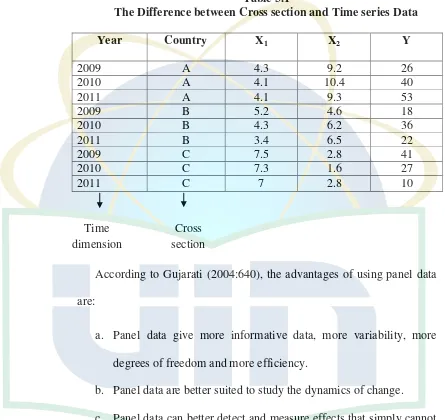
1. Credit Default Swap
[image:72.612.83.527.114.638.2]Credit Default Swap (CDS) is an instrument that had emerging at the end of the 20th century. The function of Credit Default Swap is as a tool to measure the sovereign risk. It also apply as an instrument that hedge the bond investing against the possibility of default. The following chart will shows the development of CDS market since the BIS first started reporting CDS notionals in 2004. The data provided is based on the national amount in US dollar.
Figure 4.1
Annual CDS Notionals Outstanding ($)
Source : BIS Semiannual OTC Derivatives Statistics and ISDA
$ 6.4
$ 13.9
$ 28.7
$ 58.2
$ 49.1
$ 32.7
$ 29.9 $ 28.6
$ 25.1
0 10 20 30 40 50 60 70
2004 2005 2006 2007 2008 2009 2010 2011 2012
CDS outstanding
55
International Swaps and Derivatives Association (ISDA, 2012) holds that the total notional amount of outstanding CDS contracts rose from $2,2 trillion in December of 2002 to $58.2 trillion in December of 2007. The market size had more than doubled during each of these years but hit a setback in 2008 as it suffered from worldwide financial instability.
2. Bloomberg LP
Bloomberg LP is a privately held financial software, data and media
company headquartered in New York City. Bloomberg L.P. provides financial software tools such as an analytics and equity trading platform, data services and news to financial companies and organizations through the Bloomberg terminal.
56
B. Data Description
The data processing in this research is conducted by the statistical application. The application used for data processing in this research are eviews 7th version and gretl.
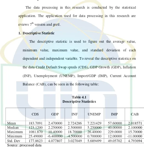
1. Descriptive Statistic
[image:74.612.90.553.124.599.2]The descriptive statistic is used to figure out the average value, minimum value, maximum value, and standard deviation of each dependent and independent variable. To reveal the descriptive statistics on the data Credit Default Swap spreds (CDS), GDP Growth (GDP), Inflation (INF), Unemployment (UNEMP), Import/GDP (IMP), Current Account Balance (CAB), can be seen in the following table:
Table 4.1 Descriptive Statistics
CDS GDP INF UNEMP IMP CAB
Mean 183.7091 2.470000 2.724286 7.221429 57.60000 2.018571 Median 123.1200 2.250000 2.500000 5.250000 40.00000 2.100000 Maximum 1081.870 10.40000 18.70000 26.40000 229.0000 15.70000 Minimum 25.49000 -6.400000 -4.500000 0.700000 12.00000 -11.00000 Std. Dev 177.8623 4.077807 3.027049 5.689499 49.05702 4.793694 Source: processed data
57
a. CDS Spreads
The average value of CDS spreads variable is 183.70 with the standard deviation of 177.86. The lowest value is 25.49 bps, while the highest value is 1081.87 bps.
b. GDP Growth
The average value of GDP growth variable is 2.47, with the standard deviation of 4.077. The lowest value is -6.4 percent, while the highest is 10.4 percent.
c. Inflation
The average value of inflation variable is 2.72 percent, with the standard deviation of 3.02. The lowest value is -4.5 percent, while the highest value is 18.7 percent.
d. Unemployment
The average value of unemployment variable is 7.22 percent, with the standard deviation of 5.68. The lowest value is 0.70 percent, while the highest value is 26.40 percent.
e. Import/GDP
58
f. Current Account Balance
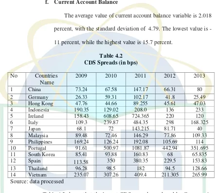
[image:76.612.92.536.116.514.2]The average value of current account balance variable is 2.018 percent, with the standard deviation of 4.79. The lowest value is -11 percent, while the highest value is 15.7 percent.
Table 4.2 CDS Spreads (in bps)
No Countries
Name
2009 2010 2011 2012 2013
1 China 73.24 67.58 147.17 66.31 80
2 Germany 26.33 59.31 102.17 41.8 25.49
3 Hong Kong 47.76 44.66 89.255 45.61 47.03
4 Indonesia 190.35 129.02 208.0 136 233
5 Ireland 158.43 608.65 724.365 220 120
6 Italy 109.3 239.87 484.35 298 168.325
7 Japan 68.1 72 143.215 81.71 40
8 Malaysia 89.48 72.46 146.29 77.86 109.33
9 Philippines 169.24 126.24 192.08 105.69 114
10 Portugal 91.61 500.97 1081.87 4