http://dx.doi.org/10.12988/ams.2014.411939
The Effects of Haze on the Spectral and Statistical
Properties of Land Cover Classification
Asmala Ahmad
Department of Industrial Computing
Faculty of Information and Communication Technology Universiti Teknikal Malaysia Melaka
Hang Tuah Jaya, 76100 Durian Tunggal, Melaka, Malaysia
Shaun Quegan
Department of Applied Mathematics School of Mathematics and Statistics
University of Sheffield Sheffield, United Kingdom
Copyright ©2014 Asmala Ahmad and Shaun Quegan. This is an open access article distributed
under the Creative Commons Attribution License, which permits unrestricted use, distribution, and reproduction in any medium, provided the original work is properly cited.
Abstract
Haze occurs almost every year in Malaysia and is caused by smoke which originates from forest fire in Indonesia. It causes visibility to drop, therefore affecting the data acquired for this area using optical sensor such as that on board Landsat satellite. The effects of haze on the data can be observed from the spectral and statistical properties of land cover classification. The work presented in this thesis is meant to analyse the statistical properties of land cover classification of hazy dataset. Maximum Likelihood (ML) was found to be a preferable classification scheme in which the effects of haze can be investigated. The study made use of hazy dataset that were simulated based on real haze spectral and statistical properties. By investigating these dataset, the spectral and statistical properties of the land classes can be systematically analysed, in which showing that haze modifies the class spectral signatures and statistical properties, consequently causing the data quality to decline.
1 Introduction
Haze reduces visibility due to the attenuation (i.e. scattering and absorption) of solar radiation by the haze constituents [13]. Most haze consists of aerosols (suspension of fine solid particles or liquid droplets in the atmosphere) and trace gases, ranging in size from a few nanometres to a few micrometers [1], [10]. Studies have shown that haze that is due to biomass burning contains large amounts of hazardous gases, i.e., carbon monoxide (CO), nitrogen dioxide (NO2) and sulphur dioxide (SO2), and particulate matter, i.e., PM10 [11], [14], [15]. Compared to gases, aerosol has a more significant impact on visibility. The largest aerosol loading from biomass burning occurs below 5 km in altitude [12]. Atmospheric scattering and absorption depend very much on the wavelength of the radiation and the size of the atmospheric constituents it interacts with. Scattering is usually much stronger for short wavelengths than long wavelengths.
Particles with size approximately 0.1 to 10 μm are particularly effective in Mie
scattering in the visible wavelength regions (0.4 – 0.7 μm) hence can impair ground level visibilities [4]. In order to quantify the effects of haze, we therefore need to identify a suitable classification method and performance criteria against which to measure these effects.
One of the primary uses of remote sensing data is to classify land covers [5], [7], [8]. A large number of classification methods are available, but our principal aim is to select the method most appropriate to the studies of haze [6], [9]. Our criteria for this selection include:
• simplicity, i.e. the practicality of using a large amount of data. This should involve a smaller number of procedures but should produce reasonably accurate and standard results,
• the ability to select important land covers with an acceptable accuracy, i.e. each pixel will be assigned to the correct land cover on the ground – the performance of the method should not be easily affected by factors such as the complexity of land covers, topographic conditions, etc. and
• objectivity, i.e. not involving tuning by a user to improve performance – the generated classification works straight away without needing any adjustment in terms of the number of classes, training pixels, etc.
(0.45-0.52 μm), band 2 (0.52-0.60 μm) and band 3 (0.63-0.69 μm), reflective infrared band 4 (0.76-0.90 μm), band 5 (1.55-1.75 μm) and band 7 (2.08-2.35
μm), with 30 m spatial resolution and thermal infrared band 6 (10.40-12.50 μm)
with 120 m spatial resolution.
This study aims to analyse the spectral and statistical properties of land cover classification of hazy dataset. The study makes used hazy dataset that were simulated based on real haze spectral and statistical properties. By using these dataset, the spectral and statistical properties of the land classes can be systematically investigated and therefore the effects of haze can be assessed. In achieving the aim, Section 2 describes ML classification of hazy dataset, Section 3 elaborates the statistical and spectral properties of Classes for the Hazy Datasets and finally, Section 4 concludes the study.
2 ML Classification on the Simulated Hazy Dataset
The vector-based structure of a dataset, the hazy band i, L V can be written as i
[9]:Li
( )
V =(
1- b i( )1( )
V)
Ti+LO+b i( )2( )
V Hi ... (1)where Ti is signal component, Hi is haze component, LO is path radiance due to natural scattering of the atmosphere, b
i 1
( ) is weighting due to signal attenuation
and b
i 2
( ) is weighting due to haze intensity.
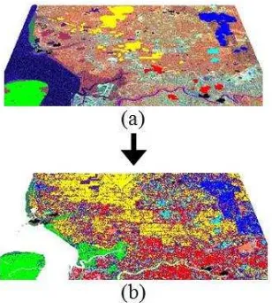
Fig. 1. (a) Patches of different colours are ROIs for different land classes used for selecting training pixels from a 4 km visibility hazy scene and (b) the ML
classification.
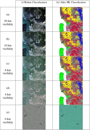
Figure 2 shows the 4 km hazy datasets before and after ML classification for visibilities 20 km, 10 km, 6 km, 4 km, 2 km and 0 km. These visibilities are chosen to visually show the transition from clear to very hazy conditions. It is obvious that the effects of haze become more severe on bands 3, 2, and 1 (assigned to the red, green and blue channels respectively) as visibility decreases (images on the left). These bands are displayed since they are more affected by the haze than the bands with longer wavelengths. Therefore, classification is much more influenced by the effects of haze in shorter than longer wavelengths. The middle images show the corresponding ML classification using training pixels from the hazy dataset itself. As expected, the ML classification performance degrades as visibility drops. The classes are clearly inseparable at 0 km visibility.
3 Spectral and Statistical Properties of Land Cover Classes in
Hazy Dataset
[image:4.595.224.378.126.297.2](i) Before Classification (ii) After ML Classification
(a) 20 km visibility
(b) 10 km visibility
(c) 6 km visibility
(d) 4 km visibility
[image:5.595.112.485.124.665.2](e) 0 km visibility
Fig. 2. Bands 3, 2 and 1 assigned to red, green and blue channels respectively (left), the ML classification using training pixels from hazy datasets (right) and ML classification using training pixels from clear datasets for (a) 20 km (clear),
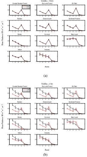
the original class radiance (red curve) and hazy class radiance (black curve) is very small for most classes. Similarly, there is little difference between the standard deviation of the original class radiance (red vertical bars) and the hazy class radiance (black vertical bars). At 2 km visibility, the haze clearly increases the radiance of bands 1, 2 and 3 for most classes except for bare land and industry, which decrease. The increase in radiance tends to occur for dark classes (e.g. forests and vegetation) because the apparent radiance is dominated by the haze radiance (i.e. radiance scattered directly to the satellite’s field of view). A decrease in radiance tends to occur for bright classes because the haze scatters
some of the solar radiance out of the satellite’s field of view before reaching the
ground, and attenuates the reflected radiation on the way back. These effects become more apparent as haze severity increases. This is consistent with Equation (1) that shows that haze increases L V through the scattering effects on i
2
i V Hi
but at the same time decreases L V through the absorption effects i
on
1 i1
V
Ti. Hence, the absorption effect is proportional to T ; therefore i the brighter the surface, the higher the absorption, consequently the more L Vi
decreases. However, it should be noted that this is true in absolute terms but not relative; i1
V does not depend on T .It can also be seen that most classes i exhibit an increase in standard deviation as visibility reduces. In other words, the haze increases the variability in the intensity of the class pixels and consequently leads to an increase in the pixels’ standard deviation. This is expected from Equation (1); since:
1 2
i i i i i
1 2 1 2
i i i i i i i i
Var L V Var 1 V T V H
= Var 1 V T Var V H 2C 1 V T , V H
+
i
T is independent of H , so the third term equal to zero. However we cannot i discard the T term since the target is not constant, so there still exist some i variance.
2
2
1 2
i i i i i
Var L V = 1 V Var T V Var H
1 2 3 4 5 7 0
50
100 Coastal Swamp Forest
Clear 16 km
1 2 3 4 5 7 0
50
100 Dry Land Forest
1 2 3 4 5 7 0
50
100 Oil Palm
1 2 3 4 5 7 0
50 100
Rubber
1 2 3 4 5 7 0
50 100
Cleared Land
1 2 3 4 5 7 0
50 100
Sediment Plumes
1 2 3 4 5 7 0
50
100 Water
1 2 3 4 5 7 0
50
100 Coconut
1 2 3 4 5 7 0
50
100 Bare Land
1 2 3 4 5 7 0
50 100
Urban
1 2 3 4 5 7 0 50 100 Industry Band M e a n R a d ia n ce ( W m
-2 sr
-1
m
-1)
Visibility = 16 km
(a)
1 2 3 4 5 7
0 50
100 Coastal Swamp Forest
Clear 2 km
1 2 3 4 5 7
0 50
100 Dry Land Forest
1 2 3 4 5 7
0 50
100 Oil Palm
1 2 3 4 5 7
0 50 100
Rubber
1 2 3 4 5 7
0 50 100
Cleared Land
1 2 3 4 5 7
0 50 100
Sediment Plumes
1 2 3 4 5 7
0 50 100
Water
1 2 3 4 5 7
0 50 100
Coconut
1 2 3 4 5 7
0 50 100
Bare Land
1 2 3 4 5 7
0 50
100 Urban
1 2 3 4 5 7
0 50 100 Industry Band M e a n R a d ia n ce ( W m
-2 sr
-1
m
-1)
Visibility = 2 km
[image:7.595.148.434.130.643.2](b)
Fig. 3. Mean radiances versus bands of individual classes for a scene with haze (black) and without haze (red) at visibility (a) 16 and (b) 2 km. Vertical bars
indicate standard deviations.
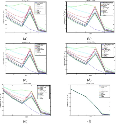
their true spectral signature curves, but experience little modification by haze at 16 and 12 km visibility. At 4 visibility, these curves are severely modified by the haze and become inseparable as the visibility reduces to 0 km. At 0 km visibility, all curves become very close, approximating the pure haze spectral signature. In other words, during no or light haze, the spectral signature of the classes are evident because the true signal radiance predominates, but as the haze gets severe, the spectral signature of the classes vanishes and is replaced by that of pure haze.
1 2 3 4 5 7
0 10 20 30 40 50 60 70 80 Band R a d ia n ce ( W m
-2 sr
-1
m
-1)
Visibility = 20 km
Coastal Swamp Forest Dryland Forest Oil Palm Rubber Cleared Land Sediment Plumes Coconut Water Bare Land Urban Industry
1 2 3 4 5 7
0 10 20 30 40 50 60 70 80 Band R a d ia n ce ( W m
-2 sr
-1
m
-1)
Visibility = 16 km
Coastal Swamp Forest Dryland Forest Oil Palm Rubber Cleared Land Sediment Plumes Coconut Water Bare Land Urban Industry
(a) (b)
1 2 3 4 5 7
0 10 20 30 40 50 60 70 80 Band R a d ia n ce ( W m
-2 sr
-1
m
-1)
Visibility = 12 km
Coastal Swamp Forest Dryland Forest Oil Palm Rubber Cleared Land Sediment Plumes Coconut Water Bare Land Urban Industry
1 2 3 4 5 7
0 10 20 30 40 50 60 70 Band R a d ia n ce ( W m
-2 sr
-1
m
-1)
Visibility = 6 km
Coastal Swamp Forest Dryland Forest Oil Palm Rubber Cleared Land Sediment Plumes Coconut Water Bare Land Urban Industry
(c) (d)
1 2 3 4 5 7
0 10 20 30 40 50 60 70 Band R a d ia n ce ( W m
-2 sr
-1
m
-1)
Visibility = 4 km
Coastal Swamp Forest Dryland Forest Oil Palm Rubber Cleared Land Sediment Plumes Coconut Water Bare Land Urban Industry
1 2 3 4 5 7
0 20 40 60 80 100 120 140 Band R a d ia n ce ( W m
-2 sr
-1
m
-1)
Visibility = 0 km
Coastal Swamp Forest Dryland Forest Oil Palm Rubber Cleared Land Sediment Plumes Coconut Water Bare Land Urban Industry
[image:8.595.115.484.240.637.2](e) (f)
Fig. 4. Mean spectral signatures of the 12 classes at visibilities (a) 20, (b) 16, (c) 12, (d) 6, (e) 4 and (f) 0 km.
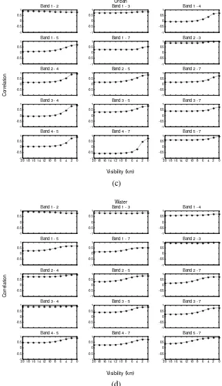
For each class, correlations between different band pairs were computed for visibilities running from 20 km to 0 km from the simulated hazy datasets by using
agreement. The correlation between band k and band l of a simulated radiance scene with a particular visibility V can be expressed by the following equation:
S
C L V, k, l
ρ k,l
Var L V, k Var L V, l
... (2)
1 1 2 2
k l k l
2
1 2 2
k k
where
C L V, k, l 1 V 1 V C T k, l V V C H k, l and
Var L V, k 1 V Var T k V Var H k , and
C T k, l , Var T k
and Var T l
are measured from the clear datasetwhileC H k, l
, Var H k
and Var H l
are measured from the pure haze dataset. Here, we assume β V k1
and β k2
V are constant throughout the image.Plots of correlation against visibility for coastal swamp forest, oil palm, urban and water are shown in Figure 5(a-e). Correlations at 20 km visibility represent the
classes’ original correlation during clear sky condition (i.e. no haze); the
-1 -0.5 0 0.5 1
Band 1 - 2
-1 -0.5 0 0.5 1
Band 1 - 3
-1 -0.5 0 0.5 1
Band 1 - 4
-1 -0.5 0 0.5 1
Band 1 - 5
-1 -0.5 0 0.5 1
Band 1 - 7
-1 -0.5 0 0.5 1
Band 2 - 3
-1 -0.5 0 0.5 1
Band 2 - 4
-1 -0.5 0 0.5 1
Band 2 - 5
-1 -0.5 0 0.5 1
Band 2 - 7
-1 -0.5 0 0.5 1
Band 3 - 4
-1 -0.5 0 0.5 1
Band 3 - 5
-1 -0.5 0 0.5 1
Band 3 - 7
20 18 16 14 12 10 8 6 4 2 0
-1 -0.5 0 0.5 1
Band 4 - 5
20 18 16 14 12 10 8 6 4 2 0
-1 -0.5 0 0.5 1
Band 4 - 7
20 18 16 14 12 10 8 6 4 2 0
-1 -0.5 0 0.5 1
Band 5 - 7
Visibility (km) C o rre la ti o n
Coastal Swamp Forest
(a) -1 -0.5 0 0.5 1
Band 1 - 2
-1 -0.5 0 0.5 1
Band 1 - 3
-1 -0.5 0 0.5 1
Band 1 - 4
-1 -0.5 0 0.5 1
Band 1 - 5
-1 -0.5 0 0.5 1
Band 1 - 7
-1 -0.5 0 0.5 1
Band 2 - 3
-1 -0.5 0 0.5 1
Band 2 - 4
-1 -0.5 0 0.5 1
Band 2 - 5
-1 -0.5 0 0.5 1
Band 2 - 7
-1 -0.5 0 0.5 1
Band 3 - 4
-1 -0.5 0 0.5 1
Band 3 - 5
-1 -0.5 0 0.5 1
Band 3 - 7
20 18 16 14 12 10 8 6 4 2 0
-1 -0.5 0 0.5 1
Band 4 - 5
20 18 16 14 12 10 8 6 4 2 0
-1 -0.5 0 0.5 1
Band 4 - 7
20 18 16 14 12 10 8 6 4 2 0
-1 -0.5 0 0.5 1
Band 5 - 7
-1 -0.5 0 0.5 1
Band 1 - 2
-1 -0.5 0 0.5 1
Band 1 - 3
-1 -0.5 0 0.5 1
Band 1 - 4
-1 -0.5 0 0.5 1
Band 1 - 5
-1 -0.5 0 0.5 1
Band 1 - 7
-1 -0.5 0 0.5 1
Band 2 - 3
-1 -0.5 0 0.5 1
Band 2 - 4
-1 -0.5 0 0.5 1
Band 2 - 5
-1 -0.5 0 0.5 1
Band 2 - 7
-1 -0.5 0 0.5 1
Band 3 - 4
-1 -0.5 0 0.5 1
Band 3 - 5
-1 -0.5 0 0.5 1
Band 3 - 7
20 18 16 14 12 10 8 6 4 2 0
-1 -0.5 0 0.5 1
Band 4 - 5
20 18 16 14 12 10 8 6 4 2 0
-1 -0.5 0 0.5 1
Band 4 - 7
20 18 16 14 12 10 8 6 4 2 0
-1 -0.5 0 0.5 1
Band 5 - 7
Visibility (km) C o rre la ti o n Urban (c) -1 -0.5 0 0.5 1
Band 1 - 2
-1 -0.5 0 0.5 1
Band 1 - 3
-1 -0.5 0 0.5 1
Band 1 - 4
-1 -0.5 0 0.5 1
Band 1 - 5
-1 -0.5 0 0.5 1
Band 1 - 7
-1 -0.5 0 0.5 1
Band 2 - 3
-1 -0.5 0 0.5 1
Band 2 - 4
-1 -0.5 0 0.5 1
Band 2 - 5
-1 -0.5 0 0.5 1
Band 2 - 7
-1 -0.5 0 0.5 1
Band 3 - 4
-1 -0.5 0 0.5 1
Band 3 - 5
-1 -0.5 0 0.5 1
Band 3 - 7
20 18 16 14 12 10 8 6 4 2 0
-1 -0.5 0 0.5 1
Band 4 - 5
20 18 16 14 12 10 8 6 4 2 0
-1 -0.5 0 0.5 1
Band 4 - 7
20 18 16 14 12 10 8 6 4 2 0
-1 -0.5 0 0.5 1
Band 5 - 7
[image:11.595.128.451.132.693.2]Visibility (km) C o rre la ti o n Water (d)
4 Conclusions
In this study, we successfully quantified the spectral and statistical properties of land cover classification under hazy conditions. Maximum Likelihood (ML) is found to be the preferable classification scheme in which the effects of haze were investigated. The study made use of hazy dataset that were simulated based on real haze spectral and statistical properties. By investigating these dataset, the spectral and statistical properties of the land classes were systematically analysed, in which showing that haze modifies the class spectral signatures and statistical properties, consequently causing the quality of the dataset to decline.
Acknowledgments. We would like to thank Universiti Teknikal Malaysia Melaka
(UTeM) for funding this study under UTeM PJP Grant (PJP/2013/FTMK(4A)/S01 146).
References
[1] A. Ahmad and M. Hashim, Determination of haze using NOAA-14 satellite data, Proceedings on The 23rd Asian Conference on Remote Sensing 2002 (ACRS 2002), (2012).
[2] A. Ahmad and S. Quegan, Analysis of maximum likelihood classification on multispectral data, Applied Mathematical Sciences, 6 (2012), 6425 – 6436. [3] A. Ahmad and S. Quegan, Analysis of maximum likelihood classification technique on Landsat 5 TM satellite data of tropical land covers, Proceedings of 2012 IEEE International Conference on Control System, Computing and Engineering (ICCSCE2012), (2012), 1 – 6.
http://dx.doi.org/10.1109/iccsce.2012.6487156
[4] A. Ahmad and M. Hashim, Determination of haze API from forest fire emission during the 1997 thick haze episode in Malaysia using NOAA AVHRR data, Malaysian Journal of Remote Sensing & GIS, July, 1 (2000), 77 – 84.
[5] A. Ahmad and S. Quegan, Comparative analysis of supervised and unsupervised classification on multispectral data, Applied Mathematical Sciences, 7 (74) (2013), 3681 – 3694. http://dx.doi.org/10.12988/ams.2013.34214
[6] A. Ahmad and S. Quegan, Haze reduction from remotely sensed data. Applied Mathematical Sciences, 8 (36) (2014), 1755 – 1762.
[7] U. K. Mohamad Hashim and A. Ahmad, The effects of training set size on the accuracy of maximum likelihood, neural network and support vector machine classification. Science International, 26 (4) (2014), 1477 – 1481.
[8] A. Ahmad, Analysis of Landsat 5 TM data of Malaysian land covers using ISODATA clustering technique, Proceedings of the 2012 IEEE Asia-Pacific Conference on Applied Electromagnetic (APACE 2012), (2012), 92 – 97.
http://dx.doi.org/10.1109/apace.2012.6457639
[9] A. Ahmad and S. Quegan, Haze Modelling and Simulation in Remote Sensing Satellite Data. Applied Mathematical Sciences, 8 (159) (2014), 7909 – 7921. http://dx.doi.org/10.12988/ams.2014.49761
[10] A. Asmala, M. Hashim, M. N. Hashim, M. N. Ayof and A. S. Budi, The use of remote sensing and GIS to estimate Air Quality Index (AQI) Over Peninsular Malaysia, GIS development, (2006), 5pp.
[11] A. Heil, A. and J. G. Goldammer, Smoke-haze pollution: a review of the 1997 episode in Southeast Asia. Regional Environmental Change, 2 (2001), 24 – 37. http://dx.doi.org/10.1007/s101130100021
[12] C. Chiang, W. Chen, W. Liang, S.K. Das and J. Nee, Optical properties of tropospheric aerosols based on measurements of lidar, sun-photometer, and
visibility at Chung-Li (251N, 1211E). Atmospheric Environment, 41 (2007), 4128
– 4137. http://dx.doi.org/10.1016/j.atmosenv.2007.01.019
[13] M. Hashim, K. D. Kanniah, A. Ahmad, A. W. Rasib, Remote sensing of tropospheric pollutants originating from 1997 forest fire in Southeast Asia, Asian Journal of Geoinformatics 4, 57 – 68.
[14] M. Mahmud, Mesoscale equatorial wind prediction in Southeast Asia during a haze episode of 2005. Geofizika, 26 (1) (2009), 67 – 84.
[15] M. Radojevic, Chemistry of Forest Fires and Regional Haze with Emphasis on Southeast Asia. Pure and Applied Geophysics, 160 (1) (2003), 157 – 187. http://dx.doi.org/10.1007/s00024-003-8771-x