http://dx.doi.org/10.12988/ams.2015.52157
The Effects of Haze on the Accuracy of
Satellite Land Cover Classification
Asmala Ahmad
Department of Industrial Computing
Faculty of Information and Communication Technology Universiti Teknikal Malaysia Melaka
Hang Tuah Jaya, 76100 Durian Tunggal, Melaka, Malaysia
Shaun Quegan
Department of Applied Mathematics School of Mathematics and Statistics
University of Sheffield Sheffield, United Kingdom
Copyright ©2015 Asmala Ahmad and Shaun Quegan. This is an open access article distributed under the Creative Commons Attribution License, which permits unrestricted use, distribution, and reproduction in any medium, provided the original work is properly cited.
Abstract
Keywords: Classification, Haze, Classification Accuracy, Landsat-5 TM, ML
1 Introduction
National land cover mapping projects using passive remote sensing satellite systems have been initiated by countries such as the United States of America and the United Kingdom that possess up-to-date technologies, facilities and expertise. In the USA, the National Land Cover Data (NLCD) with 300 m resolution was started in the 1990s by the Multi-Resolution Land Characteristics Consortium (MRLC), and its latest version, NLCD2001, with 30 m resolution, was completed in 2001. It used Landsat-5 TM and Landsat-7 ETM+ data. In the UK, the Land Cover Map 2000 (LCM2000) was produced by the Centre for Ecology and Hydrology in 2000 and was an upgraded version of the LCM Great Britain developed in 1990 0. The LCM2000 covers the whole Great Britain, i.e. England, Scotland, Wales and Northern Ireland with 25 m resolution. In Malaysia, since 1966, land cover maps were produced using aerial photographs by the Malaysian Department of Agriculture (DOA). The use of remote sensing technology was initiated by the Malaysian government in 1988 with the establishment of the Agensi Remote Sensing Malaysia (ARSM), under the government’s Ministry of Science, Technology and Innovation. In order to produce land cover maps, remote sensing data need to undergo classification process to distinguish between land covers that exist within an area. Due to its practicality, objectivity and simplicity, ML, a supervised classification method, has been commonly used in producing land cover maps. Nevertheless, during the end of the year, the quality of remote sensing data declines due to haze phenomenon, which consequently reduces the accuracy of land cover classification. Haze is caused by atmospheric aerosols and molecules that scatter and absorb solar radiation and thus affecting the downward and upward radiance of the solar radiation. Such scattering and absorption depend substantially on the wavelength of the electromagnetic waves that form the radiation 0 in which is stronger for short compared to long wavelengths 0, 0. In haze study, acquiring real hazy remote sensing datasets 0, 0, 0 with a desired range of haze concentrations over an area is difficult 0. A more practical way is to use real dataset that has been integrated with simulated haze 0, 0, 0. Section 2 describes the methodology of this study. In section 3, the effects of haze on the classification accuracy of the individual classes are described. Section 4 discusses the effects of haze on the overall classification accuracy. Finally, section 5 concludes this study.
2 Methodology
In this study, the area of interest is Klang, located in Selangor, Malaysia, which covers approximately 540 km2 within longitude 101° 10’ E to 101°30’ E and
latitude 2°99’ N to 3°15’ N 0. The satellite data comes from bands 1, 2, 3, 4, 5 and
land cover map from October 1991 of the study area. The map, with a 1:50,000 scale, was produced by ARSM using SPOT data dated 26 February and 10 June 1991 and was supplemented by Landsat data and a ground truth survey carried out on October 1991. For each land cover, a different set of the pixels were chosen to be the training and reference pixels. They were selected by making use of the stratified random sampling technique on the land covers that exist in the study area, i.e. rubber, coastal swamp forest, dryland forest, oil palm, industry, cleared land, urban, coconut, bare land, sediment plumes and water 0. The data were then integrated with haze layer which was earlier generated based on real haze properties 0, 0. By doing so, hazy datasets with visibilities ranging from 20 km (clear) to 0 km (pure haze) were produced 0. ML classification was then applied to these hazy datasets by making use of the training pixels extracted from the datasets themselves 0, 0. Accuracy assessment of the ML classification is determined by means of a confusion matrix, which compares, on a class-by-class basis, the relationship between reference data (ground truth) and the corresponding results of a classification 0, 0. Such matrices are square, with the number of rows and columns being equal to the number of classes, i.e. 11. From these matrices two accuracy measures namely, producer accuracy and overall accuracy were computed. Producer accuracy is a measure of the accuracy of a particular classification scheme and shows the percentage of a particular ground class that has been correctly classified. The minimum acceptable accuracy for a class is 70% 0, 0. This is calculated by dividing each of the diagonal elements in the confusion matrix by the total of the column in which it occurs:
aa
a
c Producer accuracy
c
(1)
where,
th th
aa
a
c element at position a row and a column c column sum
A measure of behaviour of the ML classification can be determined by the overall accuracy, which is the total percentage of pixels correctly classified, i.e.:
U
aa a 1
c Overall accuracy
Q
(2)3 The Effects of Haze on the Producer Accuracy of ML
Classification
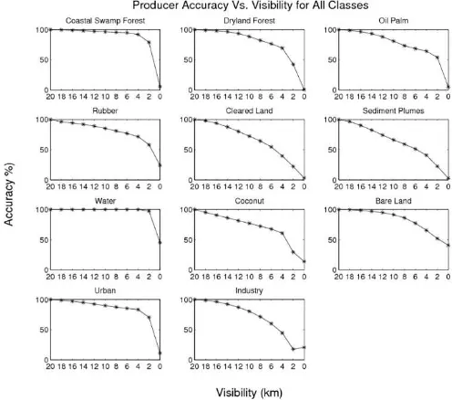
Haze modifies the means and band correlations of a class that govern the ML classification. In this section we therefore investigate how haze affects the classification accuracy of the individual classes. The assessment is carried out using the confusion matrix. Figure 1 shows producer accuracy plots for all 11 cover types. All classes show a decrease in classification accuracy as visibility reduces. Less reflective classes, such as forest, oil palm, rubber and water, experience a gradual decline at longer visibilities but then a more rapid decline at shorter visibilities. Haze starts to severely affect these classes at visibilities less than 4 km. Cleared land and sediment plumes exhibit a nearly linear decline. Some classes, i.e. rubber, water, coconut, bare land, urban and industry, exhibit a non-zero accuracy at 0 km visibility; this is because some pixels are still correctly classified to these classes because not severely influenced by very thick haze compared to other classes. For industry, an unexpected increasing trend is observed from 2 km to 0 km visibility. This is primarily because of similarity between the statistics (i.e. mean and covariance structure) of haze and industry.
Fig. 1. Producer accuracy for each class with reducing visibility.
Fig. 2. A portion of ML classification for (left) 20 km, (middle) 2 km and (right) 0 km visibility datasets (top), the corresponding enlarged versions (second row)
and enlarged versions with non-industry pixels masked in black (c).
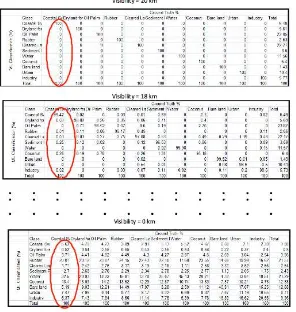
Visual inspection by simultaneously displaying the different visibility confusion matrices is not possible. A more convenient way is by plotting the elements from a particular column of the confusion matrix for each visibility (Figure 3). By doing so, the distribution of ground truth pixels assigned to the different classes as visibility changes can be analysed.
Fig. 3. Extraction of the element from a column of the confusion matrices.
highest points (referring to the percentages of correctly classified coastal swamp forest pixels at different visibilities) concentrate between 90% and 100%, for 20 km to 4 km-visibility curves, indicating that most coastal swamp forest pixels are correctly classified at good to quite poor visibilities. A similar case is observed for water. Hence, haze has little effect on these classes even when it is quite severe. For other classes (i.e. dryland forest, oil palm, rubber, coconut, bare land and urban) that are more affected by the haze, the peaks are less concentrated. The classes most affected are cleared land, sediment plumes and industry, in which the peak is only about 40% for 4 km visibility. An upward trend in the plots represents the pixels being misclassified to other classes as the visibility reduces. This happens because, when haze exists, the pixels tend to migrate to incorrect classes, as summarised in Table 1. Due to the very distinct spectral properties of water, almost no migration of water pixels occurs at all visibilities except 0 km. For most classes, the pixels tend to migrate to a single class. Coastal swamp forest, water, coconut, bare land, urban and industry pixels are likely to migrate to sediment plumes, rubber, oil palm, industry, cleared land and urban classes respectively. Dryland forest, oil palm and rubber pixels tend to migrate to the coconut class. The cleared land and sediment plumes pixels tend to migrate to multiple classes, which are oil palm, rubber, coconut and urban for the former, and forests and coconut for the latter.
Table 1: The main incorrect classes to which the pixels migrate as visibility reduces. The grey shaded boxes are not relevant for this analysis.
Ground Truth Pixels
Incorrect ML Class which the pixels fall into Coastal
Swamp Forest
Dryland Forest
Oil
Palm Rubber
Cleared Land
Sediment
Plumes Water Coconut Bare
land Urban Industry Coastal
Swamp Forest
Dryland
Forest
Oil Palm
Rubber
Cleared
Land
Sediment
Plumes
Water
Coconut
Bare
Land
Urban
Industry
suggests that the modification of spectral properties of these classes due to very thick haze is not as severe as other classes.
(i) (j)
(k)
Fig. 4. Percentage of pixels for (a) coastal swamp forest, (b) dryland forest, (c) oil palm, (d) rubber, (e) cleared land, (f) sediment plumes, (g) water, (h) coconut, (i)
bare land, (j) urban and (k) industry, against ground truth classes. 100% for a given class type, represents all the pixels from that class.
4 The Effects of Haze on the Overall Accuracy of ML
Classification
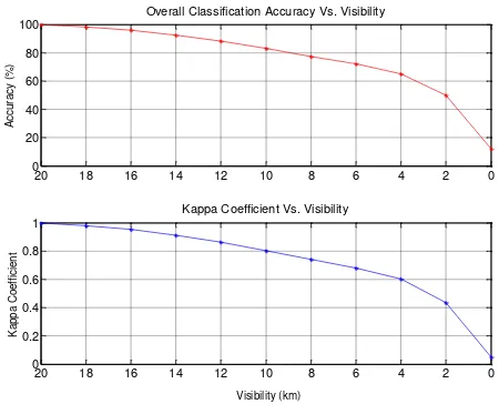
Figure 5 shows a plot of overall classification accuracy and kappa coefficient against visibility; both decline as visibility drops. The classification accuracy degrades at a faster rate as visibility gets poorer. The haze becomes intolerable at visibilities less than about 11 km (i.e. 85% accuracy). For 8 km visibility (moderate haze), accuracy reduces by about 20%. About 70% drop in accuracy occurs between 8 and 0 km visibility. A much sharper decline can be observed for visibilities less than 4 km, with only 50% classification accuracy remaining at about 2 km visibility. It is clear that the kappa coefficient plot shows a consistent result with the classification accuracy plot.
Fig. 5. Overall classification accuracy (top) and Kappa coefficient (bottom) versus visibility.
5 Conclusion
In this study, we initially performed ML classification on hazy Landsat-5 TM datasets over Selangor Malaysia to classify 11 classes i.e. rubber, coastal swamp forest, dryland forest, oil palm, industry, cleared land, urban, coconut, bare land, sediment plumes and water. ML classification was carried out for visibilities ranging from 20 km (clear) to 0 km (pure haze). The accuracy of the classification was computed using confusion matrices where the accuracy of individual classes and overall accuracy were determined for each of the hazy datasets. Further analysis was carried out in terms of visual inspection and distribution of ground truth pixels assigned to the different classes as visibility changes. The result shows that in overall, classification accuracy declines faster as visibility gets poorer. The study also reveals that the effects of haze on the accuracy of individual classes vary depending on their spectral properties.
Acknowledgments. We thank Universiti Teknikal Malaysia Melaka (UTeM) for
funding this study under UTeM PJP Grant (PJP/2013/FTMK(4A)/S01146).
References
[1] A. Ahmad and M. Hashim, Determination of haze using NOAA-14 satellite data, Proceedings on The 23rd Asian Conference on Remote Sensing 2002 (ACRS 2002), (2012), in cd.
[2] A. Ahmad and S. Quegan, Analysis of maximum likelihood classification on
20 18 16 14 12 10 8 6 4 2 0
0 20 40 60 80 100
Accu
ra
cy
(%
)
Overall Classification Accuracy Vs. Visibility
20 18 16 14 12 10 8 6 4 2 0
0 0.2 0.4 0.6 0.8 1
Ka
p
p
a
C
o
e
ff
ici
e
n
t
Kappa Coefficient Vs. Visibility
multispectral data, Applied Mathematical Sciences, 6 (2012), 6425 – 6436.
[3] A. Ahmad and S. Quegan, Analysis of maximum likelihood classification technique on Landsat 5 TM satellite data of tropical land covers, Proceedings of 2012 IEEE International Conference on Control System, Computing and Engineering (ICCSCE2012), (2012), 1 – 6.
http://dx.doi.org/10.1109/iccsce.2012.6487156
[4] A. Ahmad and S. Quegan, Cloud masking for remotely sensed data using spectral and principal components analysis, Engineering, Technology & Applied Science Research (ETASR), 2 (2012), 221 – 225.
[5] A. Ahmad and S. Quegan, Comparative analysis of supervised and unsupervised classification on multispectral data, Applied Mathematical Sciences, 7(74) (2013), 3681 – 3694. http://dx.doi.org/10.12988/ams.2013.34214
[6] A. Ahmad et al. Haze reduction from remotely sensed data. Applied Mathematical Sciences, 8(36) (2014), 1755 – 1762.
http://dx.doi.org/10.12988/ams.2014.4289
[7] A. Ahmad and S. Quegan, Multitemporal cloud detection and masking using MODIS data, Applied Mathematical Sciences, 8(7) (2014), 345 – 353.
http://dx.doi.org/10.12988/ams.2014.311619
[8] A. Ahmad, Analysis of Landsat 5 TM data of Malaysian land covers using ISODATA clustering technique, Proceedings of the 2012 IEEE Asia-Pacific Conference on Applied Electromagnetic (APACE 2012), (2012), 92 – 97.
http://dx.doi.org/10.1109/apace.2012.6457639
[9] A. Asmala, M. Hashim, M. N. Hashim, M. N. Ayof and A. S. Budi, The use of remote sensing and GIS to estimate Air Quality Index (AQI) Over Peninsular Malaysia, GIS development, (2006), 5pp.
[10] A. Ahmad and S. Quegan, Haze modelling and simulation in remote sensing satellite data, Applied Mathematical Sciences, 8(159) (2014), 7909 – 7921.
http://dx.doi.org/10.12988/ams.2014.49761
[11] C. Y. Ji, Haze reduction from the visible bands of LANDSAT TM and ETM+ images over a shallow water reef environment, Remote Sensing of Environment, 112 (2008), 1773 – 1783.
http://dx.doi.org/10.1016/j.rse.2007.09.006
http://dx.doi.org/10.1109/36.581987
[13] G. D. Moro and L. Halounova, Haze removal for high-resolution satellite data: a case study. Int. J. on Remote Sensing, 28(10) (2007), 2187 – 2205.
http://dx.doi.org/10.1080/01431160600928559
[14] M. Hashim, K. D. Kanniah, A. Ahmad, A. W. Rasib, Remote sensing of tropospheric pollutants originating from 1997 forest fire in Southeast Asia, Asian Journal of Geoinformatics 4, 57 – 68.
[15] R. M. Fuller, R. Cox, R. T. Clarke, P. Rothery, R. A. Hill, G. M. Smith, A. G. Thomson, N. J. Brown, D. C. Howard and A. P. Stott, The UK land cover map 2000: Planning, construction and calibration of a remotely sensed, user-oriented map of broad habitats, International Journal of Applied Earth Observation and Geoinformation, 7(3) (2005), 202 – 216.
http://dx.doi.org/10.1016/j.jag.2005.04.002
[16] S. Y. Kotchenova, E. F. Vermote, R. Matarrese and F. J. Klemm Jr., Validation of a vector version of the 6S radiative transfer code for atmospheric correction of satellite data. Part I: Path Radiance, Applied Optics, 45(26) 2006, 6726 – 6774. http://dx.doi.org/10.1364/ao.45.006762
[17] Y. J. Kaufman and C. Sendra, Algorithm for automatic atmospheric corrections to visible and near-IR satellite imagery, International Journal on Remote Sensing, 9(8) (1988), 1357 – 1381.
http://dx.doi.org/10.1080/01431168808954942
[18] Y. J. Kaufman and R. S. Fraser, Different atmospheric effects in remote sensing of uniform and nonuniform surfaces, Advances in Space Research, 2(5) (1982), 147 – 155. http://dx.doi.org/10.1016/0273-1177(82)90342-8